Solve PDE with Discontinuity

This example shows how to solve a PDE that interfaces with a material. The material interface creates a discontinuity in the problem at $\mathit{x}=0.5$, and the initial condition has a discontinuity at the right boundary $\mathit{x}=1$.

Consider the piecewise PDE

$$\{\begin{array}{cc}\frac{\partial \mathit{u}}{\partial \mathit{t}}={\mathit{x}}^{-2}\frac{\partial }{\partial \mathit{x}}\left({\mathit{x}}^{2}5\frac{\partial \mathit{u}}{\partial \mathit{x}}\right)-1000{\mathit{e}}^{\mathit{u}}& \left(0\le \mathit{x}\le 0.5\right)\\ \frac{\partial \mathit{u}}{\partial \mathit{t}}={\mathit{x}}^{-2}\frac{\partial }{\partial \mathit{x}}\left({\mathit{x}}^2\frac{\partial \mathit{u}}{\partial \mathit{x}}\right)-{\mathit{e}}^{\mathit{u}}& \left(0.5\le \mathit{x}\le 1\right)\end{array}$$

The initial conditions are

$$\begin{array}{l}\mathit{u}\left(\mathit{x},0\right)=0\left(0\le \mathit{x}<1\right),\\ \mathit{u}\left(1,0\right)=1\left(\mathit{x}=1\right).\end{array}$$

The boundary conditions are

$$\begin{array}{l}\frac{\partial \mathit{u}}{\partial \mathit{x}}=0\left(\mathit{x}=0\right),\\ \mathit{u}\left(1,\mathit{t}\right)=1\left(\mathit{x}=1\right).\end{array}$$

To solve this equation in MATLAB®, you need to code the equation, the initial conditions, and the boundary conditions, then select a suitable solution mesh before calling the solver pdepe. You either can include the required functions as local functions at the end of a file (as done here), or save them as separate, named files in a directory on the MATLAB path.

Code Equation

Before you can code the equation, you need to make sure that it is in a form that the pdepe solver expects. The standard form that pdepe expects is

$\mathit{c}\left(\mathit{x},\mathit{t},\mathit{u},\frac{\partial \mathit{u}}{\partial \mathit{x}}\right)\frac{\partial \mathit{u}}{\partial \mathit{t}}={\mathit{x}}^{-\mathit{m}}\frac{\partial }{\partial \mathit{x}}\left({\mathit{x}}^{\mathit{m}}\mathit{f}\left(\mathit{x},\mathit{t},\mathit{u},\frac{\partial \mathit{u}}{\partial \mathit{x}}\right)\right)+\mathit{s}\left(\mathit{x},\mathit{t},\mathit{u},\frac{\partial \mathit{u}}{\partial \mathit{x}}\right)$.

In this case, the PDE is in the proper form, so you can read off the values of the coefficients.

$\{\begin{array}{cc}\frac{\partial \mathit{u}}{\partial \mathit{t}}={\mathit{x}}^{-2}\frac{\partial }{\partial \mathit{x}}\left({\mathit{x}}^{2}5\frac{\partial \mathit{u}}{\partial \mathit{x}}\right)-1000{\mathit{e}}^{\mathit{u}}& \left(0\le \mathit{x}\le 0.5\right)\\ \frac{\partial \mathit{u}}{\partial \mathit{t}}={\mathit{x}}^{-2}\frac{\partial }{\partial \mathit{x}}\left({\mathit{x}}^2\frac{\partial \mathit{u}}{\partial \mathit{x}}\right)-{\mathit{e}}^{\mathit{u}}& \left(0.5\le \mathit{x}\le 1\right)\end{array}$

The values for the flux term $\mathit{f}\left(\mathit{x},\mathit{t},\mathit{u},\frac{\partial \mathit{u}}{\partial \mathit{x}}\right)$ and source term $\mathit{s}\left(\mathit{x}.\mathit{t},\mathit{u},\frac{\partial \mathit{u}}{\partial \mathit{x}}\right)$ change depending on the value of $\mathit{x}$. The coefficients are:

$$\mathit{m}=2$$

$$\mathit{c}\left(\mathit{x},\mathit{t},\mathit{u},\frac{\partial \mathit{u}}{\partial \mathit{x}}\right)=1$$

$$\{\begin{array}{cc}\mathit{f}\left(\mathit{x},\mathit{t},\mathit{u},\frac{\partial \mathit{u}}{\partial \mathit{x}}\right)=5\frac{\partial \mathit{u}}{\partial \mathit{x}}& \left(0\le \mathit{x}\le 0.5\right)\\ \mathit{f}\left(\mathit{x},\mathit{t},\mathit{u},\frac{\partial \mathit{u}}{\partial \mathit{x}}\right)=\frac{\partial \mathit{u}}{\partial \mathit{x}}& \left(0.5\le \mathit{x}\le 1\right)\end{array}$$

$$\{\begin{array}{cc}\mathit{s}\left(\mathit{x},\mathit{t},\mathit{u},\frac{\partial \mathit{u}}{\partial \mathit{x}}\right)=-1000{\mathit{e}}^{\mathit{u}}& \left(0\le \mathit{x}\le 0.5\right)\\ \mathit{s}\left(\mathit{x},\mathit{t},\mathit{u},\frac{\partial \mathit{u}}{\partial \mathit{x}}\right)=-{\mathit{e}}^{\mathit{u}}& \left(0.5\le \mathit{x}\le 1\right)\end{array}$$

Now you can create a function to code the equation. The function should have the signature [c,f,s] = pdex2pde(x,t,u,dudx):

• x is the independent spatial variable.

• t is the independent time variable.

• u is the dependent variable being differentiated with respect to x and t.

• dudx is the partial spatial derivative $\partial \mathit{u}/\partial \mathit{x}$.

• The outputs c, f, and s correspond to coefficients in the standard PDE equation form expected by pdepe. These coefficients are coded in terms of the input variables x, t, u, and dudx.

As a result, the equation in this example can be represented by the function:

function [c,f,s] = pdex2pde(x,t,u,dudx)
c = 1;
if x <= 0.5
    f = 5*dudx;
    s = -1000*exp(u);
else
    f = dudx;
    s = -exp(u);
end
end

(Note: All functions are included as local functions at the end of the example.)

Code Initial Conditions

Next, write a function that returns the initial conditions. The initial condition is applied at the first time value and provides the value of $\mathit{u}\left(\mathit{x},{\mathit{t}}_0\right)$ for any value of $\mathit{x}$. Use the function signature u0 = pdex2ic(x) to write the function.

The initial conditions are

$$\begin{array}{l}\mathit{u}\left(\mathit{x},0\right)=0\left(0\le \mathit{x}<1\right),\\ \mathit{u}\left(1,0\right)=1\left(\mathit{x}=1\right).\end{array}$$

The corresponding function is

function u0 = pdex2ic(x)
if x < 1
    u0 = 0;
else
    u0 = 1;
end
end

Code Boundary Conditions

Now, write a function that evaluates the boundary conditions. For problems posed on the interval $\mathit{a}\le \mathit{x}\le \mathit{b}$, the boundary conditions apply for all t and either $\mathit{x}=\mathit{a}$ or $\mathit{x}=\mathit{b}$. The standard form for the boundary conditions expected by the solver is

$$\mathit{p}\left(\mathit{x},\mathit{t},\mathit{u}\right)+\mathit{q}\left(\mathit{x},\mathit{t}\right)\mathit{f}\left(\mathit{x},\mathit{t},\mathit{u},\frac{\partial \mathit{u}}{\partial \mathit{x}}\right)=0.$$

Since this example has spherical symmetry ($\mathit{m}=2$), the pdepe solver automatically enforces the left boundary condition to bound the solution at the origin, and ignores any conditions specified for the left boundary in the boundary function. So for the left boundary condition, you can specify ${\mathit{p}}_{\mathit{L}}={\mathit{q}}_{\mathit{L}}=0$. For the right boundary condition, you can rewrite the boundary condition in the standard form and read off the coefficient values for ${\mathit{p}}_{\mathit{R}}$ and ${\mathit{q}}_{\mathit{R}}$.

For $\mathit{x}=1$, the equation is $\mathit{u}\left(1,\mathit{t}\right)=1\to \left(\mathit{u}-1\right)+0\cdot \frac{\partial \mathit{u}}{\partial \mathit{x}}=0$. The coefficients are:

• $${\mathit{p}}_{\mathit{R}}\left(1,\mathit{t},\mathit{u}\right)=\mathit{u}-1$$

• $${\mathit{q}}_{\mathit{R}}\left(1,\mathit{t}\right)=0$$

The boundary function should use the function signature [pl,ql,pr,qr] = pdex2bc(xl,ul,xr,ur,t):

• The inputs xl and ul correspond to u and x for the left boundary.

• The inputs xr and ur correspond to u and x for the right boundary.

• t is the independent time variable.

• The outputs pl and ql correspond to ${\mathit{p}}_{\mathit{L}}\left(\mathit{x},\mathit{t},\mathit{u}\right)$ and ${\mathit{q}}_{\mathit{L}}\left(\mathit{x},\mathit{t}\right)$ for the left boundary ($\mathit{x}=0$ for this problem).

• The outputs pr and qr correspond to ${\mathit{p}}_{\mathit{R}}\left(\mathit{x},\mathit{t},\mathit{u}\right)$ and ${\mathit{q}}_{\mathit{R}}\left(\mathit{x},\mathit{t}\right)$ for the right boundary ($\mathit{x}=1$ for this problem).

The boundary conditions in this example are represented by the function:

function [pl,ql,pr,qr] = pdex2bc(xl,ul,xr,ur,t)
pl = 0; 
ql = 0; 
pr = ur - 1;
qr = 0;
end

Select Solution Mesh

The spatial mesh should include several values near $\mathit{x}=0.5$ to account for the discontinuous interface, as well as points near $\mathit{x}=1$ because of the inconsistent initial value ($\mathit{u}\left(1,0\right)=1$) and boundary value ($\mathit{u}\left(1,\mathit{t}\right)=0$) at that point. The solution changes rapidly for small $\mathit{t}$, so use a time step that can resolve this sharp change.

x = [0 0.1 0.2 0.3 0.4 0.45 0.475 0.5 0.525 0.55 0.6 0.7 0.8 0.9 0.95 0.975 0.99 1];
t = [0 0.001 0.005 0.01 0.05 0.1 0.5 1];

Solve Equation

Finally, solve the equation using the symmetry m, the PDE equation, the initial conditions, the boundary conditions, and the meshes for x and t.

m = 2;
sol = pdepe(m,@pdex2pde,@pdex2ic,@pdex2bc,x,t);

pdepe returns the solution in a 3-D array sol, where sol(i,j,k) approximates the kth component of the solution ${\mathit{u}}_{\mathit{k}}$ evaluated at t(i) and x(j). The size of sol is length(t)-by-length(x)-by-length(u0), since u0 specifies an initial condition for each solution component. For this problem, u has only one component, so sol is a 8-by-18 matrix, but in general you can extract the kth solution component with the command u = sol(:,:,k).

Extract the first solution component from sol.

u = sol(:,:,1);

Plot Solution

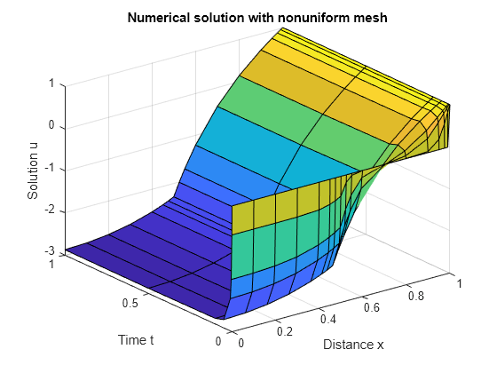
Create a surface plot of the solution $\mathit{u}$ plotted at the selected mesh points for $\mathit{x}$ and $\mathit{t}$. Since $\mathit{m}=2$ the problem is posed in a spherical geometry with spherical symmetry, so the solution only changes in the radial $\mathit{x}$ direction.

surf(x,t,u)
title('Numerical solution with nonuniform mesh')
xlabel('Distance x')
ylabel('Time t')
zlabel('Solution u')

Now, plot just $\mathit{x}$ and $\mathit{u}$ to get a side view of the contours in the surface plot. Add a line at $\mathit{x}=0.5$ to highlight the effect of the material interface.

plot(x,u,x,u,'*')
line([0.5 0.5], [-3 1], 'Color', 'k')
xlabel('Distance x')
ylabel('Solution u')
title('Solution profiles at several times')

Local Functions

Listed here are the local helper functions that the PDE solver pdepe calls to calculate the solution. Alternatively, you can save these functions as their own files in a directory on the MATLAB path.

function [c,f,s] = pdex2pde(x,t,u,dudx) % Equation to solve
c = 1;
if x <= 0.5
    f = 5*dudx;
    s = -1000*exp(u);
else
    f = dudx;
    s = -exp(u);
end
end
%----------------------------------------------
function u0 = pdex2ic(x) %Initial conditions
if x < 1
    u0 = 0;
else
    u0 = 1;
end
end
%----------------------------------------------
function [pl,ql,pr,qr] = pdex2bc(xl,ul,xr,ur,t) % Boundary conditions
pl = 0;
ql = 0;
pr = ur - 1;
qr = 0;
end
%----------------------------------------------