Rotational Transformations on the Globe
In The Orientation Vector, you explored the concept of altering the aspect of a map projection in terms of pushing the North Pole to new locations. Another way to think about this is to redefine the coordinate system, and then to compute a normal aspect projection based on the new system. For example, you might redefine a spherical coordinate system so that your home town occupies the origin. If you calculated a map projection in a normal aspect with respect to this transformed coordinate system, the resulting display would look like an oblique aspect of the true coordinate system of latitudes and longitudes.
This transformation of coordinate systems can be useful independent of map displays. If you transform the coordinate system so that your home town is the new North Pole, then the transformed coordinates of all other points will provide interesting information.
Note
The types of coordinate transformations described here are appropriate for the spherical case only. Attempts to perform them on an ellipsoid will produce incorrect answers on the order of several to tens of meters.
When you place your home town at a pole, the spherical distance of each point from your hometown becomes 90° minus its transformed latitude (also known as a colatitude). The point antipodal to your town would become the South Pole, at -90°. Its distance from your hometown is 90°-(-90°), or 180°, as expected. Points 90° distant from your hometown all have a transformed latitude of 0°, and thus make up the transformed equator. Transformed longitudes correspond to their respective great circle azimuths from your home town.
Reorient Vector Data with rotatem
The rotatem function uses an orientation vector to transform
latitudes and longitudes into a new coordinate system. The orientation vector can be
produced by the newpole or putpole functions, or
can be specified manually.
As an example of transforming a coordinate system, suppose you live in Midland, Texas, at (32°N,102°W). You have a brother in Tulsa (36.2°N,96°W) and a sister in New Orleans (30°N,90°W).
Define the three locations:
midl_lat = 32;   midl_lon = -102;
tuls_lat = 36.2; tuls_lon = -96;
newo_lat = 30;   newo_lon = -90;
Use the
distancefunction to determine great circle distances and azimuths of Tulsa and New Orleans from Midland:[dist2tuls az2tuls] = distance(midl_lat,midl_lon,... tuls_lat,tuls_lon) dist2tuls = 6.5032 az2tuls = 48.1386 [dist2neworl az2neworl] = distance(midl_lat,midl_lon,... newo_lat,newo_lon) dist2neworl = 10.4727 az2neworl = 97.8644Tulsa is about 6.5 degrees distant, New Orleans about 10.5 degrees distant.
Compute the absolute difference in azimuth, a fact you will use later.
azdif = abs(az2tuls-az2neworl)

azdif =
   49.7258
Today, you feel on top of the world, so make Midland, Texas, the north pole of a transformed coordinate system. To do this, first determine the origin required to put Midland at the pole using
newpole:origin = newpole(midl_lat,midl_lon) origin = 58 78 0
The origin of the new coordinate system is (58°N, 78°E). Midland is now at a new latitude of 90°.
Determine the transformed coordinates of Tulsa and New Orleans using the
rotatemcommand. Because its units default to radians, be sure to include thedegreeskeyword:[tuls_lat1,tuls_lon1] = rotatem(tuls_lat,tuls_lon,... origin,'forward','degrees') tuls_lat1 = 83.4968 tuls_lon1 = -48.1386 [newo_lat1,newo_lon1] = rotatem(newo_lat,newo_lon,... origin,'forward','degrees') newo_lat1 = 79.5273 newo_lon1 = -97.8644Show that the new colatitudes of Tulsa and New Orleans equal their distances from Midland computed in step 2 above:
tuls_colat1 = 90-tuls_lat1

tuls_colat1 =
    6.5032

newo_colat1 = 90-newo_lat1

newo_colat1 =
   10.4727
Recall from step 4 that the absolute difference in the azimuths of the two cities from Midland was 49.7258°. Verify that this equals the difference in their new longitudes:
tuls_lon1-newo_lon1

ans =
   49.7258
You might note small numerical differences in the results (on the order of 10-6), due to round-off error and trigonometric functions.
For further information, see the reference pages for rotatem, newpole, putpole, neworig, and org2pol.
Reorient Gridded Data
This example shows how to transform a regular data grid into a new one with its data rearranged to correspond to a new coordinate system using the neworig function. You can transform coordinate systems of data grids as well as vector data. When regular data grids are manipulated in this manner, distance and azimuth calculations with the map variable become row and column operations.
Load elevation raster data and a geographic cells reference object. Transform the data set to a new coordinate system in which a point in Sri Lanka is the north pole. Reorient the data grid by using the neworig function. Note that the result, [Z,lat,lon], is a geolocated data grid, not a regular data grid like the original data.
load topo60c
origin = newpole(7,80);
[Z,lat,lon] = neworig(topo60c,topo60cR,origin);
Display the new map, in normal aspect, as its orientation vector shows. Note that every cell in the first row of the new grid is 0 to 1 degrees distant from the point new origin. Every cell in its second row is 1 to 2 degrees distant, and so on. In addition, every cell in a particular column has the same great circle azimuth from the new origin.
axesm miller
lat = linspace(-90,90,90);
lon = linspace(-180,180,180);
surfm(lat,lon,Z);
demcmap(topo60c)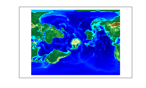
mstruct = getm(gca);
mstruct.origin
ans = 1×3

     0     0     0