avhrrgoode
Read AVHRR data product stored in Goode Projection
Syntax
[latgrat,longrat,z] = avhrrgoode(region,filename)

[...] = avhrrgoode(region,filename,scalefactor)

[...] = avhrrgoode(region,filename,scalefactor,latlim,lonlim)

[...] = avhrrgoode(region,filename,scalefactor,latlim,lonlim,gsize)

[...] = avhrrgoode(region,filename,scalefactor,latlim,lonlim,gsize,...

nrows,ncols)

[...] = avhrrgoode(region,filename,scalefactor,latlim,lonlim,gsize,...

nrows,ncols,resolution)

[...] = avhrrgoode(region,filename,scalefactor,latlim,lonlim,gsize,...

nrows,ncols,resolution,precision)
Description
[latgrat,longrat,z] = avhrrgoode(region,filename)
reads data from an Advanced Very High Resolution Radiometer (AVHRR) data set with a nominal
resolution of 1 km that is stored in the Goode projection. Data in this format includes a
nondimensional vegetation index (NDVI) and Global Land Cover Characteristics (GLCC) data
sets. region specifies the geographic coverage of the file, using the
following values:
'g'or'global''af'or'africa''ap'or'australia/pacific''ea'or'eurasia''na'or'north america''sa'or'south america'
filename is a string scalar or character vector
specifying the name of the data file. Output Z is a geolocated data grid
with coordinates latgrat and longrat in units of
degrees. Z, latgrat, and longrat
are of class double. Projected coordinates that lie within the interrupted areas of the
projection are set to NaN. A scale factor of 100 is applied to the original data set, so
that Z contains every 100th point in both X
and Y directions.
[...] = avhrrgoode(region,filename,scalefactor) uses
the integer scalefactor to downsample the data.
A scale factor of 1 returns every point. A scale factor of 10 returns
every 10th point. The default value is
100.
[...] = avhrrgoode(region,filename,scalefactor,latlim,lonlim) returns
data for the specified region. The returned data can extend somewhat
beyond the requested area. Limits are two-element vectors in units
of degrees, with latlim in the range [-90
90] and lonlim in the range [-180
180]. latlim and lonlim must
be ascending. If latlim and lonlim are
empty, the entire area covered by the data file is returned. If the
quadrangle defined by latlim and lonlim (when
projected to form a polygon in the appropriate Goode projection) fails
to intersect the bounding box of the data in the projected coordinates,
then Z, latgrat, and longrat are
returned as empty.
[...] = avhrrgoode(region,filename,scalefactor,latlim,lonlim,gsize) controls
the size of the graticule matrices. gsize is a
two-element vector containing the number of rows and columns desired.
By default, latgrat, and longrat have
the same size as Z.
[...] = avhrrgoode(region,filename,scalefactor,latlim,lonlim,gsize,... overrides the dimensions for the
standard file format for the selected region. This syntax is useful
for data stored on CD-ROM, which may have been truncated to fit.
Some global data sets were distributed with 16347 rows and 40031 columns
of data on CD-ROMs. The default size for global data sets is 17347
rows and 40031 columns of data.
nrows,ncols)
[...] = avhrrgoode(region,filename,scalefactor,latlim,lonlim,gsize,...reads
a data set with the spatial resolution specified in meters. Specify
nrows,ncols,resolution)resolution as
either 1000 or 8000 (meters).
If empty, the full resolution of 1000 meters is assumed. Data is also
available at 8000-meter resolution. Nondimensional vegetation index
data at 8-km spatial resolution has 2168 rows and 5004 columns.
[...] = avhrrgoode(region,filename,scalefactor,latlim,lonlim,gsize,... reads
a data set expecting the integer
nrows,ncols,resolution,precision)precision specified.
If empty, 'uint8' is assumed. 'uint16' is
appropriate for some files. Check the metadata (.txt or README)
file in the GLCC ftp folder for specification of
the file format and contents. In either case, Z is
converted to class double.
Background
The United States maintains a family of satellite-based sensors
to measure climate change under the Earth Observing System (EOS) program.
The precursors to the EOS data are the data sets produced by NOAA
and NASA under the Pathfinder program. These are data derived from
the Advanced High Resolution Radiometer sensor flown on the NOAA Polar
Orbiter satellites, NOAA-7, -9, and -11, and have spatial resolutions
of about 1 km. The data from the AVHRR sensor is processed into separate
land, sea, and atmospheric indices. Land area data is processed to
a nondimensional vegetation index (NDVI) or land cover classification
and stored in binary files in the Plate Carrée, Goode, and Lambert
projections. Sea data is processed to surface temperatures and stored
in HDF formats. avhrrgoode reads land data saved
in the Goode projection with global and continental coverage at 1
km. It can also read 8 km data with global coverage.
Limitations
Most files store the data in scaled integers. Though this function returns the data as double, the scaling from integer to float is not performed. Check the data's README file for the appropriate scaling parameters.
Examples
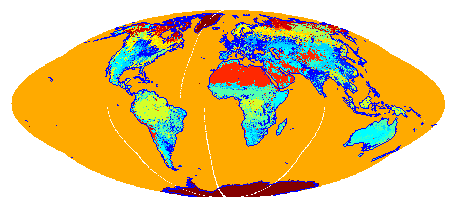
Read and display every 50th point from the Global Land Cover Characteristics
(GLCC) file covering the entire globe with the USGS classification scheme, named
gusgs2_0g.img. (To run the example, you must first download
the file.)
[latgrat, longrat, Z] = avhrrgoode('global', ...
   'gusgs2_0g.img',50);

% Convert the geolocated data grid to an geolocated image.
uniqueClasses = unique(Z);
RGB = ind2rgb8(uint8(Z), jet(numel(uniqueClasses)));

% Display the data as an image using the Goode projection.
origin = [0 0 0];
ellipsoid = [6370997 0];
figure
axesm('MapProjection', 'goode', 'Origin', origin, ...
   'Geoid', ellipsoid)
geoshow(latgrat, longrat, RGB, 'DisplayType', 'image');
axis image off

% Plot the coastlines.
hold on
load coastlines
plotm(coastlat,coastlon)
Read and display every point from the Global Land Cover Characteristics (GLCC)
file covering California with the USGS classification scheme, named
nausgs1_2g.img. You must first download the file to run this example.
figure
usamap california
mstruct = gcm;
latlim = mstruct.maplatlimit;
lonlim = mstruct.maplonlimit;
scalefactor = 1;
[latgrat, longrat, Z] = ...
   avhrrgoode('na', 'nausgs1_2g.img', scalefactor, latlim, lonlim);
geoshow(latgrat, longrat, Z, 'DisplayType', 'texturemap');

% Overlay vector data from usastatehi.shp.
california = shaperead('usastatehi', 'UseGeoCoords', true,...
   'BoundingBox', [lonlim;latlim]);
geoshow([california.Lat], [california.Lon], 'Color', 'black');

Tips
This function reads the binary files as is. You should not use byte-swapping software on these files.
The AVHRR project and data sets are described in and provided by various US Government Web sites. For more information, see the entries for Global Land Cover Characteristics (GLCC) on the Find Geospatial Raster Data page.
Version History
Introduced before R2006a