Classify Mangroves Using Sentinel-2 Multispectral Images
R2026bThis example shows how to train a DeepLab v3+ semantic segmentation network, using Sentinel-2 Level 2A multispectral images and Global Mangrove Watch (GMW) data, for pixel-level classification of mangrove regions.
Mangroves are critical to healthy coastal ecosystems. They harbor rich biodiversity, shelter numerous plant and animal species, and act as natural buffers against erosion and storm surges. However, mangrove forests are declining due to climate change and human activity, creating an urgent need for scalable monitoring and conservation tools.
Sentinel-2 Level 2A data is multispectral data acquired in the Sentinel-2 mission. The Sentinel-2 mission under the Copernicus program offers medium-resolution Earth imagery to track the variability in the conditions of the land surface of the Earth. The wide swath width and high revisit time of the mission facilitate the monitoring of changes on the surface of the Earth. Sentinel-2 Level 2A data contains 12 bands of image data having resolutions of 10 meters, 20 meters, and 60 meters. The size of a 10-meter resolution tile is 10,980-by-10,980 pixels.
This example first shows you how to perform semantic segmentation using a pretrained network to segment Sentinel-2 data based on mangrove cover. The pretrained network is a DeepLab v3+ network fine-tuned on a pretrained ResNet-50 backbone. Then, you can optionally fine-tune the pretrained network backbone on new Sentinel-2 data. This example runs best on a CUDA capable NVIDIA GPU. Use of a GPU requires Parallel Computing Toolbox. For more information about the supported compute capabilities, see GPU Computing Requirements (Parallel Computing Toolbox).
This example requires the Hyperspectral Imaging Library for Image Processing Toolbox™. You can install the Hyperspectral Imaging Library for Image Processing Toolbox from Add-On Explorer. For more information about installing add-ons, see Get and Manage Add-Ons. The Hyperspectral Imaging Library for Image Processing Toolbox requires desktop MATLAB®, as MATLAB® Online™ and MATLAB® Mobile™ do not support the library.
Download Pretrained Network
Download the pretrained network.
zipFile = matlab.internal.examples.downloadSupportFile("image","data/MangroveCoverClassificationModel.zip");
filepath = fileparts(zipFile);
unzip(zipFile,filepath)
Load the pretrained network into the workspace.
filename = fullfile(filepath,"MangroveCoverClassificationModel","MangroveCoverClassificationModel.mat");
model = load(filename);
net = model.net;
Download and Preprocess Test Data
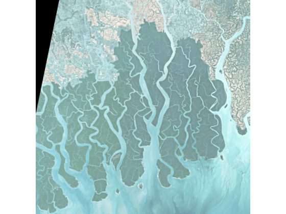
Download a Sentinel-2 Level 2A tile from the year 2020 with less than 6% cloud coverage. If you do not already have an account on the Copernicus Data Space website, create one. Download the tile into a folder named data in the current working directory. This example uses the S2B_MSIL2A_20201227T043209_N0500_R133_T45QYE_20230228T184515.SAFE tile.
Resampling all spectral bands to 10-meter resolution and assemble them into a multispectral data cube.
testFile = fullfile("data","S2B_MSIL2A_20201227T043209_N0500_R133_T45QYE_20230228T184515.SAFE","manifest.safe");
mcube = geomulticube(testFile);
resampledMcube = resampleBands(mcube,mcube.BandResolution(2));
testImgCube = gather(resampledMcube);
testImg = colorize(resampledMcube);
Visualize the test image.
imageshow(testImg)
Predict Segmentation for Test Data
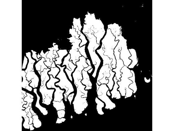
Predict mangrove regions for the test data using the predictMangrove helper function, attached to this example as a supporting file. The helper function divides the input image into 1024-by-1024 patches, predicts each patch using the trained network, and stitches the results into a full-size binary mask.
predTestImg = predictMangrove(testImgCube,net);
imageshow(predTestImg)
The rest of this example shows how to fine-tune the pretrained network backbone using new Sentinel-2 Level 2A tiles and Global Mangrove Watch (GMW) Data.
Download Training Data Sets
This example uses two data sets: Sentinel-2 satellite imagery and Global Mangrove Watch (GMW) polygon data.
Global Mangrove Watch (GMW) Data
Register on JAXA's Earth Observation Research Center website to download the GMW data. Download the GMW version 3.0 data for 2020 from the to the current working directory as a zip file named gmw_v3_2020_vec.zip. Extract the downloaded archive.
unzip("gmw_v3_2020_vec.zip")The GMW data set provides a comprehensive global record of mangrove extents as polygon geometries. Version 3.0 identifies approximately 147,359 km of mangroves in 2020 at 25-meter pixel spacing, with an accuracy of 87.4%. The data is available as a shapefile with binary classification (mangrove or non-mangrove).
Sentinel-2 Imagery
If you do not already have an account on the Copernicus Data Space website, create one. Download 22 Sentinel-2 Level 2A tiles from the year 2020 with less than 6% cloud coverage. Select images from diverse continental regions to capture global variation. Download the tiles into a folder named data in the current working directory. This example uses these Sentinel-2 Level 2A tiles.
S2A_MSIL2A_20200614T045701_N0500_R119_T44PLR_20230329T141514.SAFES2A_MSIL2A_20200614T045701_N0500_R119_T44PMR_20230329T141514.SAFES2A_MSIL2A_20201213T155521_N0500_R011_T17QRG_20230226T144454.SAFES2A_MSIL2A_20201219T160701_N0500_R097_T17RMJ_20230301T084557.SAFES2A_MSIL2A_20201221T050221_N0500_R119_T44PMC_20230327T205443.SAFES2A_MSIL2A_20201221T050221_N0500_R119_T44QPD_20230327T205443.SAFES2A_MSIL2A_20201226T041151_N0500_R047_T46QEG_20230228T170253.SAFES2A_MSIL2A_20201231T164711_N0500_R126_T15QVA_20230306T043808.SAFES2B_MSIL2A_20200828T045659_N0500_R119_T44PLQ_20230317T132733.SAFES2B_MSIL2A_20201214T042149_N0500_R090_T46QEH_20230226T170816.SAFES2B_MSIL2A_20201224T060249_N0500_R091_T42RUN_20230401T175159.SAFES2B_MSIL2A_20201227T043209_N0500_R133_T45QYE_20230228T184515.SAFES2B_MSIL2A_20201227T043209_N0500_R133_T45QZE_20230228T184515.SAFES2B_MSIL2A_20201227T043209_N0500_R133_T46QBL_20230228T184515.SAFES2B_MSIL2A_20201228T040149_N0500_R004_T46PGC_20230329T012249.SAFES2B_MSIL2A_20201230T044209_N0500_R033_T45QXE_20230228T162726.SAFES2B_MSIL2A_20201230T112359_N0500_R037_T28PCT_20230305T023728.SAFES2B_MSIL2A_20201230T112359_N0500_R037_T28PCU_20230305T023728.SAFES2B_MSIL2A_20201230T112359_N0500_R037_T28PDT_20230305T023728.SAFES2B_MSIL2A_20201230T162659_N0500_R040_T16QBJ_20230304T022351.SAFES2B_MSIL2A_20201231T055239_N0500_R048_T42QWK_20230331T233021.SAFES2B_MSIL2A_20201231T055239_N0500_R048_T42QXL_20230331T233021.SAFE
Load and Configure Training Data Paths
Load the paths to the Sentinel-2 manifest files using the loadSentinel2Data helper function, attached to this example as a supporting file. The helper function searches the data folder for all subfolders and returns a cell array of file paths to the manifest.safe file in each subfolder. Also, read the GMW shapefile into a geospatial table.
The subsequent sections of this example can be time-consuming. You can run each section independently. Execute these setup commands before running any section.
sentinelFiles = loadSentinel2Data();
numImages = numel(sentinelFiles);
gmwShapefile = "gmw_v3_2020_vec.shp";
S = readgeotable(gmwShapefile);
Preprocess Sentinel-2 Training Data
Process each Sentinel-2 tile by resampling all spectral bands to 10-meter resolution and assembling them into a multispectral data cube. The preprocessing performs these operations for each tile.
Resamples each band image to match the 10-meter resolution tile.
Concatenates all band images into a multispectral data cube of size 10,980-by-10,980-by-12.
Save each data cube as a .mat file and a truecolor rendering as a .tif file.
outFolder = "image";
mkdir(outFolder);
for numI = 1:numImages
    mcube = geomulticube(sentinelFiles{numI});
    resampledMcube = resampleBands(mcube,mcube.BandResolution(2));
    imgCube = gather(resampledMcube);
    img = colorize(resampledMcube);
    filename1 = sprintf("image%03d.mat",numI);
    save(fullfile(outFolder,filename1),"imgCube","-v7.3");
    filename2 = sprintf("image%03d.tif",numI);
    imwrite(img,fullfile(outFolder,filename2));
    disp("Image " + numI + " written to file");
    if numI==12
        sampleImg = img;
    end
end
Image 1 written to file
Image 2 written to file
Image 3 written to file
Image 4 written to file
Image 5 written to file
Image 6 written to file
Image 7 written to file
Image 8 written to file
Image 9 written to file
Image 10 written to file
Image 11 written to file
Image 12 written to file
Image 13 written to file
Image 14 written to file
Image 15 written to file
Image 16 written to file
Image 17 written to file
Image 18 written to file
Image 19 written to file
Image 20 written to file
Image 21 written to file
Image 22 written to file
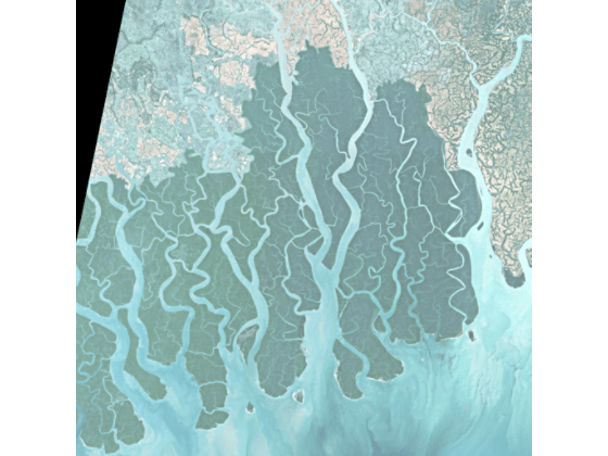
Visualize a sample truecolor image.
imageshow(sampleImg)
Create Label Masks
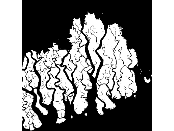
Generate binary label masks that indicate mangrove pixels for each Sentinel-2 tile. This process has two stages.
Stage 1: Identify Overlapping Polygons
For each tile, determine its geographic bounding box, then find which GMW polygons intersect with that extent. Save the polygon indices for use in mask generation.
polygonIndices = cell(1,numImages);
for numI = 1:numImages
    info = geomulticube(sentinelFiles{numI});
    [xLimits,yLimits] = deal(info.Metadata.RasterReference(2).XWorldLimits, ...
        info.Metadata.RasterReference(2).YWorldLimits);
    sentinelCRS = info.Metadata.RasterReference(2).ProjectedCRS;
    [lat,lon] = projinv(sentinelCRS,xLimits,yLimits);
    latLims(numI,:) = lat;
    lonLims(numI,:) = lon;
end
indProgPct = 0;
for i = 1:height(S)
    indProg = i/height(S)*100;
    if round(indProg) > indProgPct
        indProgPct = indProgPct + 1;
        disp("Progress: " + indProgPct + "%")
    end
    geopoly = S.Shape(i);
    for numI = 1:numImages
        poly = geoclip(geopoly,latLims(numI,:),lonLims(numI,:));
        if poly.NumRegions > 0
            polygonIndices{numI}(end+1) = i;
        end
    end
end
Progress: 1%
Progress: 2%
Progress: 3%
Progress: 4%
Progress: 5%
Progress: 6%
Progress: 7%
Progress: 8%
Progress: 9%
Progress: 10%
Progress: 11%
Progress: 12%
Progress: 13%
Progress: 14%
Progress: 15%
Progress: 16%
Progress: 17%
Progress: 18%
Progress: 19%
Progress: 20%
Progress: 21%
Progress: 22%
Progress: 23%
Progress: 24%
Progress: 25%
Progress: 26%
Progress: 27%
Progress: 28%
Progress: 29%
Progress: 30%
Progress: 31%
Progress: 32%
Progress: 33%
Progress: 34%
Progress: 35%
Progress: 36%
Progress: 37%
Progress: 38%
Progress: 39%
Progress: 40%
Progress: 41%
Progress: 42%
Progress: 43%
Progress: 44%
Progress: 45%
Progress: 46%
Progress: 47%
Progress: 48%
Progress: 49%
Progress: 50%
Progress: 51%
Progress: 52%
Progress: 53%
Progress: 54%
Progress: 55%
Progress: 56%
Progress: 57%
Progress: 58%
Progress: 59%
Progress: 60%
Progress: 61%
Progress: 62%
Progress: 63%
Progress: 64%
Progress: 65%
Progress: 66%
Progress: 67%
Progress: 68%
Progress: 69%
Progress: 70%
Progress: 71%
Progress: 72%
Progress: 73%
Progress: 74%
Progress: 75%
Progress: 76%
Progress: 77%
Progress: 78%
Progress: 79%
Progress: 80%
Progress: 81%
Progress: 82%
Progress: 83%
Progress: 84%
Progress: 85%
Progress: 86%
Progress: 87%
Progress: 88%
Progress: 89%
Progress: 90%
Progress: 91%
Progress: 92%
Progress: 93%
Progress: 94%
Progress: 95%
Progress: 96%
Progress: 97%
Progress: 98%
Progress: 99%
Progress: 100%
save("indices.mat","polygonIndices");
Stage 2: Generate Binary Masks
Convert the overlapping GMW polygons into pixel-level binary masks for each tile using the geopolyarray2polyshape and convertPolyshapeToMask helper functions, attached to this example as supporting files. The geopolyarray2polyshape function projects geographic polygons into the tile coordinate system. The convertPolyshapeToMask function rasterizes the projected polygons into a binary image matching the tile dimensions.
load indices.mat
outFolder = "label";
mkdir(outFolder);
warning("off","MATLAB:polyshape:repairedBySimplify");
for numI = 1:numImages
    info = geomulticube(sentinelFiles{numI});
    [xLimits,yLimits] = deal(info.Metadata.RasterReference(2).XWorldLimits, ...
        info.Metadata.RasterReference(2).YWorldLimits);
    sentinelCRS = info.Metadata.RasterReference(2).ProjectedCRS;
    resampledMcube = resampleBands(info,info.BandResolution(2));
    coloredImage = colorize(resampledMcube);
    numRows = size(coloredImage,1);
    numCols = size(coloredImage,2);
    BW = false(numRows,numCols);
    for i = 1:numel(polygonIndices{numI})
        poly = S.Shape(polygonIndices{numI}(i));
        pgon = geopolyarray2polyshape(poly,sentinelCRS);
        BW = BW | convertPolyshapeToMask(pgon,[numRows,numCols],xLimits,yLimits);
    end
    mask = any(coloredImage ~= 0,3);
    BW = BW & mask;
    filename = sprintf("image%03d.tif",numI);
    imwrite(BW,fullfile(outFolder,filename));
    disp("Mask for image " + numI + " written to file")
    if numI == 12
        sampleMask = BW;
    end
end
Mask for image 1 written to file
Mask for image 2 written to file
Mask for image 3 written to file
Mask for image 4 written to file
Mask for image 5 written to file
Mask for image 6 written to file
Mask for image 7 written to file
Mask for image 8 written to file
Mask for image 9 written to file
Mask for image 10 written to file
Mask for image 11 written to file
Mask for image 12 written to file
Mask for image 13 written to file
Mask for image 14 written to file
Mask for image 15 written to file
Mask for image 16 written to file
Mask for image 17 written to file
Mask for image 18 written to file
Mask for image 19 written to file
Mask for image 20 written to file
Mask for image 21 written to file
Mask for image 22 written to file
warning("on","MATLAB:polyshape:repairedBySimplify");
Visualize the binary label mask for the sample tile.
imageshow(sampleMask)
Prepare Data for Training
Prepare the data for training a DeepLab v3+ network based on ResNet-50. Mangrove pixels typically constitute a small fraction of each satellite tile, creating an inherent class imbalance. To address this, extract balanced patches from each tile that contain a controlled ratio of positive (mangrove) and negative (non-mangrove) samples.
Specify folder paths for images, labels, training patches, and predictions. Define the patch size and the number of balanced patches to extract per image.
imgFolder = fullfile(pwd,"image");
labelFolder = fullfile(pwd,"label");
classNames = {"No","Yes"};
labelIDsGT = [0 1];
patchSize = [256 256];
numBalancedPatchesPerImage = 2000;
workRoot = fullfile(pwd,"balanced_training_cache");
patchImgDir = fullfile(workRoot,"patches_images");
patchLabDir = fullfile(workRoot,"patches_labels");
predFolder = fullfile(pwd,"predictions");
mkdir(workRoot);
mkdir(patchImgDir);
mkdir(patchLabDir);
mkdir(predFolder);
Load and sort the image and label file paths.
files = dir(fullfile(imgFolder,"*.mat"));
files = files(~[files.isdir]);
[~,idx] = sort({files.name});
files = files(idx);
imgPaths = fullfile({files.folder},{files.name});
files = dir(fullfile(labelFolder,"*.tif"));
files = files(~[files.isdir]);
[~,idx] = sort({files.name});
files = files(idx);
labelPaths = fullfile({files.folder},{files.name});
Generate balanced training patches using the writeBalancedPatches helper function, attached to this example as a supporting file. The helper function extracts patches centered on positive pixels (with at least 10% mangrove coverage) and random negative patches (with less than 1% mangrove coverage), writing each patch as a .tif file. The positiveRatio parameter controls the proportion of patches containing mangrove pixels.
writeBalancedPatches(imgPaths,labelPaths,patchImgDir,patchLabDir, ...
    patchSize,numBalancedPatchesPerImage,0.5);
Processing image 1/22... Extracted 1000 positive patches Extracted 1000 negative patches Processing image 2/22... Extracted 1000 positive patches Extracted 1000 negative patches Processing image 3/22... Extracted 1000 positive patches Extracted 1000 negative patches Processing image 4/22... Extracted 1000 positive patches Extracted 1000 negative patches Processing image 5/22... Extracted 1000 positive patches Extracted 1000 negative patches Processing image 6/22... Extracted 1000 positive patches Extracted 1000 negative patches Processing image 7/22... Extracted 1000 positive patches Extracted 1000 negative patches Processing image 8/22... Extracted 1000 positive patches Extracted 1000 negative patches Processing image 9/22... Extracted 1000 positive patches Extracted 1000 negative patches Processing image 10/22... Extracted 1000 positive patches Extracted 1000 negative patches Processing image 11/22... Extracted 1000 positive patches Extracted 1000 negative patches Processing image 12/22... Extracted 1000 positive patches Extracted 1000 negative patches Processing image 13/22... Extracted 1000 positive patches Extracted 1000 negative patches Processing image 14/22... Extracted 0 positive patches Extracted 1000 negative patches Processing image 15/22... Extracted 1000 positive patches Extracted 1000 negative patches Processing image 16/22... Extracted 1000 positive patches Extracted 1000 negative patches Processing image 17/22... Extracted 1000 positive patches Extracted 1000 negative patches Processing image 18/22... Extracted 1000 positive patches Extracted 1000 negative patches Processing image 19/22... Extracted 1000 positive patches Extracted 1000 negative patches Processing image 20/22... Extracted 1000 positive patches Extracted 1000 negative patches Processing image 21/22... Extracted 1000 positive patches Extracted 1000 negative patches Processing image 22/22... Extracted 1000 positive patches Extracted 1000 negative patches Total patches written: 43000
disp("All training patches written");All training patches written
Create an imageDatastore and a pixelLabelDatastore (Computer Vision Toolbox) for the patches of data cubes and labels, respectively.
imds = imageDatastore(patchImgDir,"FileExtensions",{".tif",".tiff"});
pxds = pixelLabelDatastore(patchLabDir,classNames,labelIDsGT, ...
    "FileExtensions",{".tif",".tiff"});
Randomly split the image and pixel label data into 60% training data, 20% validation data, and 20% test data using the partitionData helper function. The helper function is attached to this example as a supporting file.
[imdsTrain,imdsVal,imdsTest,pxdsTrain,pxdsVal,pxdsTest] = partitionData(imds,pxds);
Calculate class weights using inverse frequency to handle the class imbalance during training. Classes with fewer pixels receive higher weights, encouraging the network to learn from underrepresented mangrove regions.
disp("Calculating class weights from training data...");Calculating class weights from training data...
reset(pxdsTrain);
classPixelCounts = zeros(1,numel(classNames));
while hasdata(pxdsTrain)
    temp = read(pxdsTrain);
    mask = temp{1};
    for c = 1:numel(classNames)
        classPixelCounts(c) = classPixelCounts(c) + sum(mask(:) == classNames{c});
    end
end
reset(pxdsTrain);
classWeights = 1 ./ classPixelCounts;
classWeights = classWeights / sum(classWeights);
fprintf("Class weights: No=%.4f, Yes=%.4f\n",classWeights(1),classWeights(2));
Class weights: No=0.2305, Yes=0.7695
Combine the training image and pixel label datastores, and apply random geometric augmentation using the augmentImageAndPixelLabels helper function, attached to this example as a supporting file. The helper function applies random affine transformations including rotation, reflection, scaling, shearing, and translation to both the image and its corresponding pixel labels.
dsTrain = combine(imdsTrain,pxdsTrain);
dsTrain = transform(dsTrain,@augmentImageAndPixelLabels);
dsVal = combine(imdsVal,pxdsVal);
Define Network Architecture
Use the deeplabv3plus (Computer Vision Toolbox) function to create a DeepLab v3+ network based on ResNet-50. Modify the image input layer to support 12-channel Sentinel-2 data, instead of 3-channel RGB data, and replace the first convolutional layer to accept the new input dimensions.
numClasses = numel(classNames);
numChannels = 12;
net = deeplabv3plus(patchSize,numClasses,"resnet50");
layer = imageInputLayer([patchSize numChannels],Name="input_2", ...
    Normalization="none");
net = replaceLayer(net,"input_1",layer);
layer = convolution2dLayer([7 7],64,Name="conv1", ...
    Padding=[3 3 3 3],Stride=[2 2]);
net = replaceLayer(net,"conv1",layer);
Specify Training Options
Train the network using the Adam optimization solver. Specify the hyperparameter settings using the trainingOptions (Deep Learning Toolbox) function. Set the initial learning rate to 0.0001, the mini-batch size to 8, and train for 15 epochs. You can experiment with tuning the hyperparameters based on your available system memory.
initialLearningRate = 1e-4;
maxEpochs = 15;
minibatchSize = 8;
l2reg = 0.0005;
options = trainingOptions("adam", ...
    InitialLearnRate=initialLearningRate, ...
    L2Regularization=l2reg, ...
    MaxEpochs=maxEpochs, ...
    MiniBatchSize=minibatchSize, ...
    LearnRateSchedule="piecewise", ...
    LearnRateDropPeriod=10, ...
    LearnRateDropFactor=0.5, ...
    Shuffle="every-epoch", ...
    Plots="training-progress", ...
    VerboseFrequency=20, ...
    CheckpointPath=pwd, ...
    CheckpointFrequency=5, ...
    ValidationData=dsVal, ...
    ValidationFrequency=50, ...
    OutputNetwork="best-validation-loss", ...
    ExecutionEnvironment="gpu");
Train Network
To train the network, set the doTraining variable to true. To use a network that you have previously trained, set the doTraining variable to false. Train the network using focal crossentropy loss, defined in the modelLoss helper function, attached to this example as a supporting file. The loss function uses a gamma value of 3, which helps the network focus on hard-to-classify pixels by down-weighting well-classified examples.
doTraining =false; if doTraining net = trainnet(dsTrain,net,@modelLoss,options); save("MangroveCoverClassificationModel.mat","net"); else model = load("MangroveCoverClassificationModel.mat"); net = model.net; end
Evaluate Network on Test Data
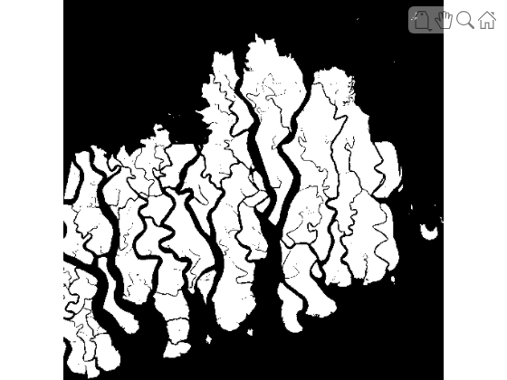
Predict mangrove regions for a selected full-size Sentinel-2 tile using the predictMangrove helper function, attached to this example as a supporting file. The helper function divides the input image into 1024-by-1024 patches, predicts each patch using the trained network, and stitches the results into a full-size binary mask.
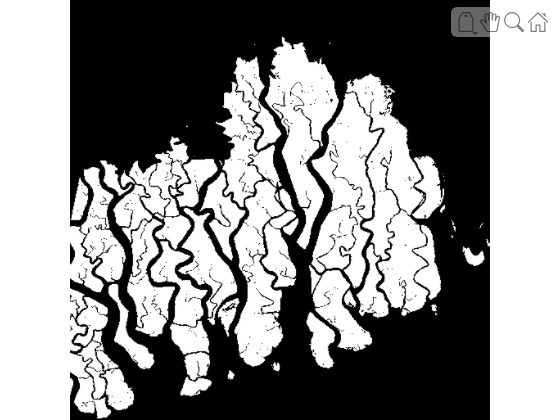
Visualize the ground truth and predicted masks for comparison.
gTruth = matlab.io.datastore.FileSet(labelFolder,"FileExtensions",".tif");
testImage = matlab.io.datastore.FileSet(imgFolder,"FileExtensions",".mat");
imgIndx = 12;
gTruthImage = imread(gTruth.FileInfo.Filename(imgIndx));
imageshow(gTruthImage)
predTestImage = predictMangrove(load(testImage.FileInfo.Filename(imgIndx)).imgCube,net);
imageshow(predTestImage)
Predict the land cover classification for the test data set using the semanticseg (Computer Vision Toolbox) function. Measure semantic segmentation performance on the test data set using the evaluateSemanticSegmentation (Computer Vision Toolbox) function.
pxdsResults = semanticseg(imdsTest,net, ...
    MiniBatchSize=4, ...
    WriteLocation=predFolder, ...
    Verbose=false, ...
    Classes=classNames);
metrics = evaluateSemanticSegmentation(pxdsResults,pxdsTest, ...
    Metrics=["global-accuracy","accuracy","weighted-iou"]);
Evaluating semantic segmentation results
----------------------------------------
* Selected metrics: global accuracy, class accuracy, weighted IoU.
* Processed 8600 images.
* Finalizing... Done.
* Data set metrics:

    GlobalAccuracy    MeanAccuracy    WeightedIoU
    ______________    ____________    ___________

        0.9226          0.89625         0.86071
Inspect the DataSetMetrics property for a high-level accuracy overview, and the ClassMetrics property for per-class performance.
disp(metrics.DataSetMetrics);
    GlobalAccuracy    MeanAccuracy    WeightedIoU
    ______________    ____________    ___________

        0.9226          0.89625         0.86071
disp(metrics.ClassMetrics);
           Accuracy
           ________

    No     0.94475
    Yes    0.84776
Save the evaluation metrics to CSV files.
try
    writetable(metrics.DataSetMetrics,fullfile(pwd,"Evaluation_DataSetMetrics.csv"));
    writetable(metrics.ClassMetrics,fullfile(pwd,"Evaluation_ClassMetrics.csv"));
catch ME
    warning("Could not write metrics CSVs: %s",ME.message);
end
References
[1] Dataset | ALOS@EORC. ALOS@EORC Homepage, https://www.eorc.jaxa.jp/ALOS/index_e.htm. Accessed 27 July 2026.
[2] Ecosystem, Copernicus Data Space. "Copernicus Data Space Ecosystem | Europe's Eyes on Earth." https://dataspace.copernicus.eu/.
See Also
imageDatastore | pixelLabelDatastore (Computer Vision Toolbox) | deeplabv3plus (Computer Vision Toolbox) | trainingOptions (Deep Learning Toolbox) | semanticseg (Computer Vision Toolbox) | evaluateSemanticSegmentation (Computer Vision Toolbox)

