Predict EV Battery Temperature Using Cascade-Correlation Model

This example shows how to simulate the battery temperature on an electric vehicle (EV) model by using a cascade-correlation neural network in a nonlinear ARX model.

Generate Input and Output Data from EV Battery Model

The EV model consists of modules such as RefSpd (the reference speed) and Passenger Car. Passenger Car includes a Simscape™ model of the battery pack. For more information, see EV Reference Application (R2024a).

To model the open-loop behavior of the battery pack, the model is adapted to isolate the pack from the cooling system. A cascade-correlation network models this battery pack. The inputs are the pack current and state-of-charge (SOC) and the output is the cell temperature.

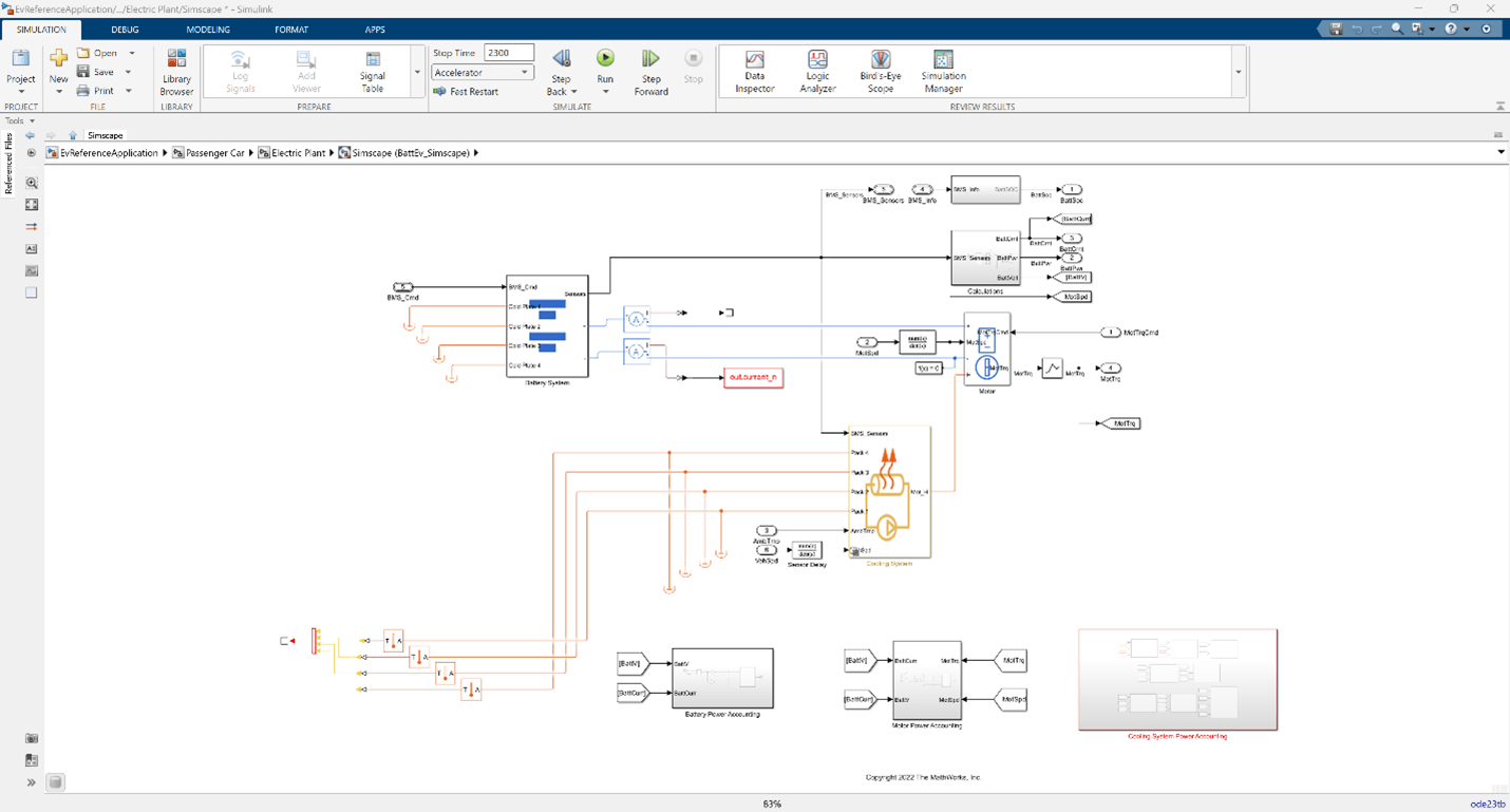
To generate realistic data, use a standardized drive cycle. You select the drive cycle, run simulations, and record the current, SOC, and temperature profile during simulation. In this process, you only vary the drive cycle and have no direct control over the current and SOC.

For this example, the cascade-correlation nonlinear ARX model is trained with the FTP-75 drive cycle simulation of 1500 seconds. To ensure that the training data is on a similar scale as the validation data, the speed is scaled by 1.2. Training data is sampled at increments of 0.1 seconds and consists of 15,001 sample points. The FTP75.mat file stores the data.

The trained model is validated with the LA-92 drive cycle simulation, which only has 1435 seconds. Validation data is also sampled at increments of 0.1 seconds and has 14,351 sample points. The LA92.mat file stores the data.

Load and Plot Data

Load the training and validation data.

rng default;
datae = load('FTP75.mat');
datav = load('LA92.mat');

Before estimating the model, inspect both the training and validation data.

eData = iddata(datae.y_temp,[datae.u_curr,datae.u_soc],0.1,'InputName',{'current','SOC'},'OutputName','temperature');
vData = iddata(datav.y_temp,[datav.u_curr,datav.u_soc],0.1,'InputName',{'current','SOC'},'OutputName','temperature');
figure()
idplot(eData,vData)
legend('Training','Validation','Location','best');

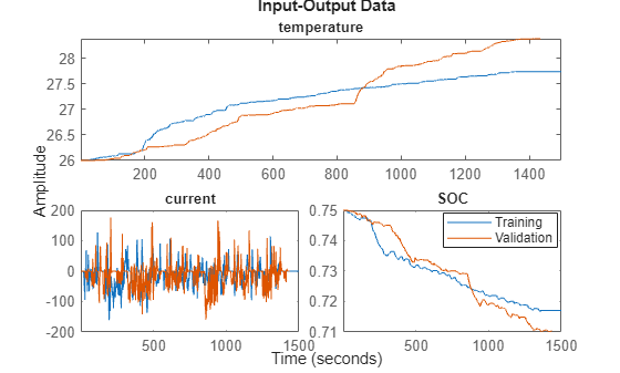
For both the current and the SOC input profiles, the training and validation data look very different. The validation data for the current and SOC inputs goes slightly outside the range of the training data, which demonstrates the model capability to generalize to an extent.

Train Model with Cross-Validation

Create the cascade-correlation neural network using idNeuralNetwork and train it using nlarx.

By default, the CrossValidate property of the nlarx option set is set to true. That is, cross-validation is enabled, which means that the software reserves part of the training data for cross-validation. You specify the percentage of cross-validation data using the CrossValidationOptions property.

After training, the software further refines the cascade-correlation network parameters using quasi-Newton methods, which is time-consuming. To suppress this refinement, set the maximum iterations of the nlarx option set to 0. You can now observe only the network performance and save time.

As you train the network, the number of activation layers increases from one to the number specified in the MaxNumActLayers name-value argument of idNeuralNetwork. For each number of activation layers, the software calculates the cross-validation residual error. Te software finally chooses the number of activation layers such that the cross-validation error is minimized.

f = idNeuralNetwork("cascade-correlation","sigmoid",0,0,MaxNumActLayers=60,SizeSelection='off');
opt = nlarxOptions;
opt.SearchOptions.MaxIterations = 0;
opt.NormalizationOptions.NormalizationMethod = 'norm';
opt.CrossValidationOptions.HoldoutFraction = 0.1;
orders = [ones(1,1),ones(1,2),ones(1,2)];
sys1 = nlarx(eData,orders,f,opt);
sys1.OutputFcn

ans = 
Multi-Layer Neural Network
Inputs: temperature(t-1), current(t-1), SOC(t-1)
Output: temperature(t)

 Nonlinear Function: Deep learning network
         Contains 32 hidden layers using "sigmoid" activations.
         (uses Deep Learning Toolbox)
 Linear Function: not in use
 Output Offset: not in use

              Network: 'Deep learning network parameters'
            LinearFcn: 'Linear function parameters'
               Offset: 'Offset parameters'
    EstimationOptions: [1×1 struct]

Compare the model performance with the training data.

figure()
compare(eData,sys1); 
title('Training Fit'); 
legend('Training Data','Model Simulation','Location','best'); 
axis([0 1500 26 28.5]);

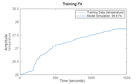
The plot shows that the model output fits the training data well.

Interactively Select Number of Layers

To interactively select the number of activation layers during training of the cascade-correlation network, set the SizeSelection name-value argument to "on".

During training, the Network Size Selection dialog box opens and shows the training and cross-validation error with respect to the number of activation layers. The dialog box also marks the layer number with the minimum cross-validation error. You can select the number of activation layers in this dialog box and click Apply.

Validate Model

Compare the model performance with the validation data.

figure()
compare(vData,sys1); 
title('Validation Fit'); 
legend('Validation Data','Model Simulation','Location','best'); 
axis([0 1500 26 28.5]);

The plot shows that the model also fits the validation data well.

Train Model with nAIC

When the CrossValidate property of the nlarx option set is set to false, the software uses all the data for training. The software uses the normalized measure of Akaike's Information Criterion (nAIC) to determine the network size. It makes a tradeoff between the fitting performance and the network size. For information on nAIC, see Model Quality Metrics.

opt.CrossValidate = false;
sys1 = nlarx(eData,orders,f,opt);
sys1.OutputFcn

ans = 
Multi-Layer Neural Network
Inputs: temperature(t-1), current(t-1), SOC(t-1)
Output: temperature(t)

 Nonlinear Function: Deep learning network
         Contains 27 hidden layers using "sigmoid" activations.
         (uses Deep Learning Toolbox)
 Linear Function: not in use
 Output Offset: not in use

              Network: 'Deep learning network parameters'
            LinearFcn: 'Linear function parameters'
               Offset: 'Offset parameters'
    EstimationOptions: [1×1 struct]

You can see that using nAIC creates a smaller network.

Compare the model performance with the training data.

figure()
compare(eData,sys1); 
title('Training Fit Without Cross-Validation'); 
legend('Training Data','Model Simulation','Location','best'); 
axis([0 1500 26 28.5]);

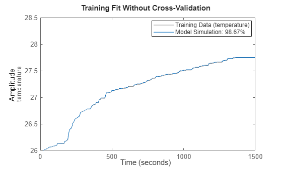
The plot shows that the smaller network still fits the training data well.

Interactively Select Number of Layers Using nAIC Metric

To interactively select the number of activation layers during training of the cascade-correlation network, set the SizeSelection name-value argument to "on".

During training, the Network Size Selection dialog box shows the training error with respect to the number of activation layers. In this example, the improvement in fit is very slow after the default number of activation layers have been added and the effects of growing network size outweighs the performance improvements. So, the nAIC metric determines the default network size of 27.

Validate Model

Compare the model performance with the validation data.

figure()
compare(vData,sys1); 
title('Validation Fit Without Cross-Validation'); 
legend('Validation Data','Model Simulation','Location','best'); 
axis([0 1500 26 28.5]);

The plot shows that the model also fits the validation data well.

In this example, the fit percentage improves when using the nAIC metric. This improvement indicates that the software overfit the model trained with cross-validation.