Electrical Load Forecasting Using AVEVA PI Asset Framework And Regression Model
This example shows how to forecast the electrical load requirement of a city using a regression model trained in MATLAB® with historical data retrieved from an AVEVA PI Asset Framework (AF) database.
Electrical load forecasting is essential for efficient energy planning and grid management. Accurate forecasting helps energy providers optimize power generation, reduce operational costs, and maintain a stable power supply by predicting demand fluctuations and avoiding grid overloads.
In this example, you retrieve five years of hourly measurements for electrical load and weather conditions from an AF database. You prepare this data to train and test a regression model. Finally, you use the trained model to predict the load requirement of a city based on weather forecast data for the upcoming two months.
This illustration shows the end-to-end workflow demonstrated in this example for electrical load forecasting.

Prerequisites
1. Install the AF SDK library to run this example. For more information, see AF SDK Overview.
2. An AVEVA PI AF server must be available on your network.
3. Access to an AF database that contains relevant attributes with time series data.
Connect to Asset Framework Server and Access AF Database
Connect to the AVEVA PI Asset Framework server using the afclient function. This example uses the Windows® computer name as the server name, which might vary depending on your PI System configuration.
host = getenv("COMPUTERNAME");
client = afclient(host);
Select the database that contains the relevant assets and data.
selectDatabase(client,"OSIDemo_PG_HydroPlant")Retrieve Historical Data of Active Power and Weather Attributes
In electrical load forecasting, load data is the target and weather conditions are predictors. Weather conditions such as ambient air temperature, precipitation, relative humidity, and wind flow speed can significantly influence electricity consumption patterns.
To retrieve historical data on electrical load usage and weather conditions of a city, first find the elements and attributes containing this data on the AF server.
In this example, the electrical load of the city is represented by the Actual Load attribute of the NYC Load Data element. Use the findAttributeByPath function to find the Actual Load attribute by its path.
attributePath = "\\BGL-SSAHA\OSIDemo_PG_HydroPlant\Flynn River Hydro\Flynn I\GU1\NYC Load Data|Actual Load";
activePowerAttribute = findAttributeByPath(client,attributePath);
Retrieve historical data for the Active Power attribute between January 1, 2020, and October 1, 2025 using the readHistory function.
startTime = datetime("01/01/2020",'InputFormat','dd/MM/uuuu');
endTime = datetime("01/10/2025",'InputFormat','dd/MM/uuuu');
loadData = readHistory(activePowerAttribute,startTime,endTime);
Extract the times and values from the retrieved data set and store them as a timetable.
loadDataValueOnly = timetable(loadData.Time,cell2mat(loadData.Value),VariableNames=activePowerAttribute.Name);
As an alternative to typing in the attribute path for the findAttributeByPath function, you can browse the element hierarchy interactively using the Asset Framework Browser. To find weather attributes, open the Asset Framework Browser and browse the element hierarchy. This example uses the weather data stored in the attributes of the NYC Weather Data element.
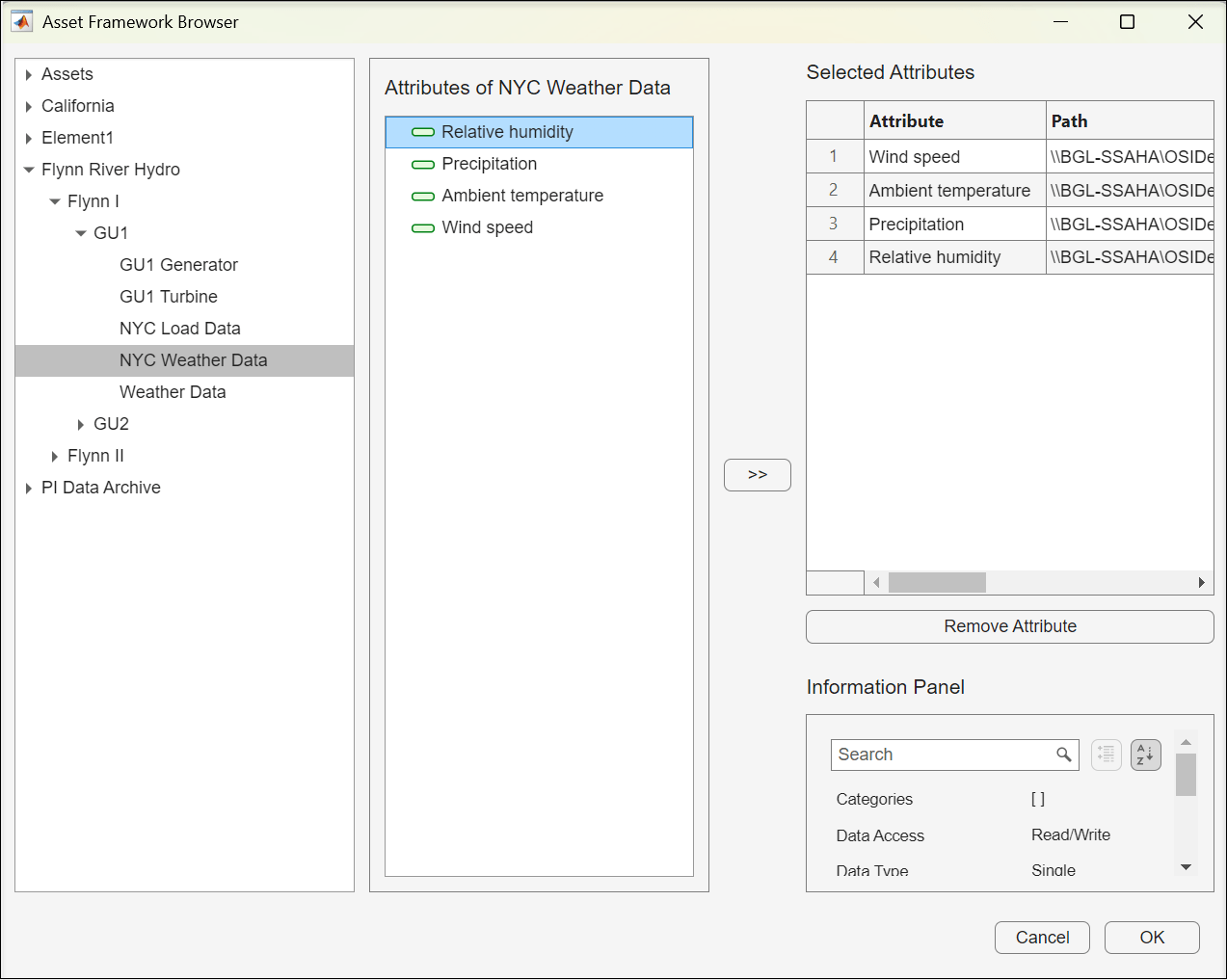
weatherAttributes = browseElements(client)
weatherAttributes =
  1×4 Attribute array:
    Index         Name                                                          Path                                                  ServerDataType
    -----  -------------------  ----------------------------------------------------------------------------------------------------  --------------
      1        Wind speed           \\BGL-SSAHA\OSIDemo_PG_HydroPlant\Flynn River Hydro\Flynn I\GU1\NYC Weather Data|Wind speed           Single
      2    Ambient temperature  \\BGL-SSAHA\OSIDemo_PG_HydroPlant\Flynn River Hydro\Flynn I\GU1\NYC Weather Data|Ambient temperature      Single
      3       Precipitation        \\BGL-SSAHA\OSIDemo_PG_HydroPlant\Flynn River Hydro\Flynn I\GU1\NYC Weather Data|Precipitation         Single
      4     Relative humidity    \\BGL-SSAHA\OSIDemo_PG_HydroPlant\Flynn River Hydro\Flynn I\GU1\NYC Weather Data|Relative humidity       Single
Preallocate cell arrays to hold weather data. Cell arrays are easier for processing because they are flexible containers that can hold different types of data. Then, loop over the number of weather attributes to retrieve data for the specified time range. Extract the time and value from each retrieved data set and store it as a timetable in the pre-allocated cell array.
ttArray = cell(size(weatherAttributes));

for idx = 1:numel(weatherAttributes)
    tt = readHistory(weatherAttributes(idx),startTime,endTime);
    ttValueOnly = timetable(tt.Time,cell2mat(tt.Value),VariableNames=weatherAttributes(idx).Name);
    ttArray{idx} = ttValueOnly;
end
Now, the cell array ttArray contains four elements, each of which is a timetable with the data from one of the four weather attributes.
Prepare Training and Test Data Sets
When each data set uses its own time vector, synchronize the data into a single timetable for accurate analysis and modeling. To create a common time basis for the retrieved data, synchronize the electrical-load and weather data into a single timetable, where each column represents the data from one attribute.
ttSynced = loadDataValueOnly;
for idx = 1:numel(ttArray)
    ttSynced = synchronize(ttSynced,ttArray{idx});
end
To see the structure of the synchronized timetable containing the electrical-load and weather data, display the first eight rows.
head(ttSynced)
                 Time                 Actual Load    Wind speed    Ambient temperature    Precipitation    Relative humidity
    ______________________________    ___________    __________    ___________________    _____________    _________________

    01-Jan-2020 00:00:00 UTC+05:30      4970.5          18.4               3.4                  0                 75
    01-Jan-2020 01:00:00 UTC+05:30      4879.4          17.6               2.1                  0                 77
    01-Jan-2020 02:00:00 UTC+05:30      4685.5            17               1.5                  0                 79
    01-Jan-2020 03:00:00 UTC+05:30      4579.5          19.4               1.2                  0                 78
    01-Jan-2020 04:00:00 UTC+05:30      4467.8          18.8               0.8                  0                 77
    01-Jan-2020 05:00:00 UTC+05:30      4452.8            18               0.6                  0                 75
    01-Jan-2020 06:00:00 UTC+05:30      4524.8          17.6               0.4                  0                 70
    01-Jan-2020 07:00:00 UTC+05:30      4648.1          15.6               1.5                  0                 75
Extract the synchronized load and weather data.
loadData = ttSynced{:,1};
weatherData = ttSynced{:,2:end};
In this example, the retrieved data set has hourly data points over a range of five years. Estimate the total number of data points based on this range. Then divide the data into training and test sets. Use 90% of the data for training and 10% for testing.
numTotalData = numel(weatherData(:,1));
numTrainData = round(numTotalData*0.9);
numTestData = numTotalData - numTrainData;

weatherDataTrain = weatherData(1:numTrainData,:);
weatherDataTest = weatherData(numTrainData+1:end,:);
In electrical load forecasting, time-based predictors such as month of the year, hour of the day, and day of the week provide interesting observations on load consumption. For example, electricity demand typically peaks in the evenings, differs between weekdays and weekends, and rises during summer and winter due to heating and cooling needs.
To include the time-based predictors for the training model, extract timestamps from the retrieved data set and divide them into training and test data sets.
timestampData = ttSynced.Time;
timestampDataTrain = timestampData(1:numTrainData);
timestampDataTest  = timestampData(numTrainData+1:end);
Extract the month, hour, and weekday information for the training and test data sets.
monthDataTrain = month(timestampDataTrain);
hourDataTrain = hour(timestampDataTrain);
weekdayDataTrain = weekday(timestampDataTrain);

monthDataTest = month(timestampDataTest);
hourDataTest = hour(timestampDataTest);
weekdayDataTest = weekday(timestampDataTest);
To obtain the final training and test data sets, combine the data sets of weather-based and time-based predictors.
XTrain = [weatherDataTrain,monthDataTrain,hourDataTrain,weekdayDataTrain];
XTest = [weatherDataTest,monthDataTest,hourDataTest,weekdayDataTest];
Similarly, extract load values for training and test data sets
YTrain = loadData(1:numTrainData,:);
YTest  = loadData(numTrainData+1:end);
Train Regression Model
Open the Regression Learner (Statistics and Machine Learning Toolbox) app with the prepared predictor matrix XTrain and the target vector YTrain.To train a regression model, use the training options in the app.
regressionLearner(XTrain,YTrain);
The trained model used in this example was created with these steps:
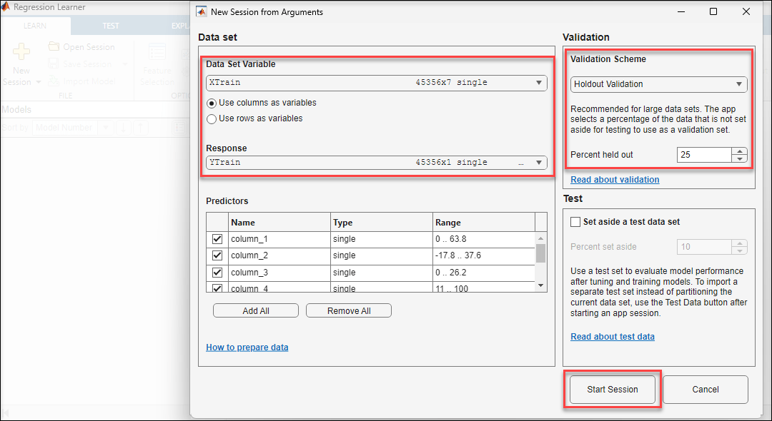
1. In the New Session from Arguments dialog box, verify the Data Set Variable and Response. Select Holdout Validation scheme and click Start Session.
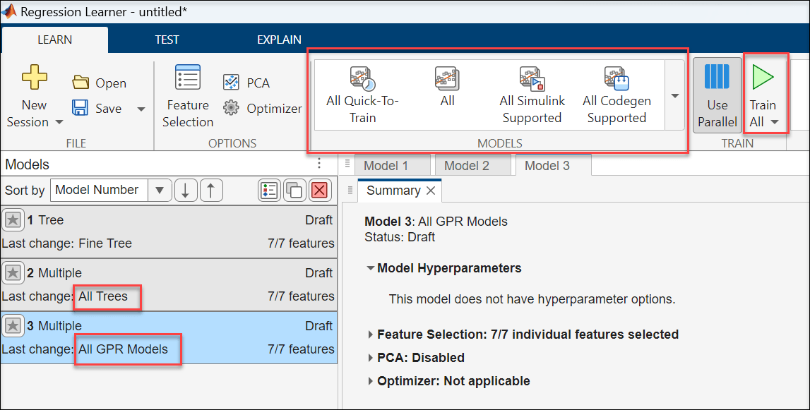
2. The app starts a new session with the provided data set and displays the response plot. To train the data with specific models, select the training models from the Models section in the Learn tab. This example uses All Trees and All GPR Models. When you select a model, it appears in the Models panel on the left. To start training, on the toolstrip, click Train All.
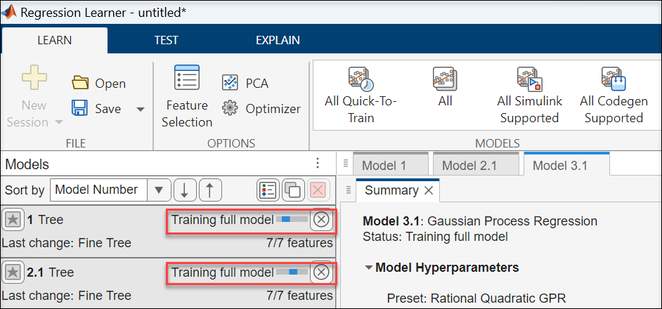
3. Wait for training to complete.
4. After the training is complete, select the model with the least RMSE and export it to the workspace. For the data set used in this example the Exponential GPR model has the least RMSE.
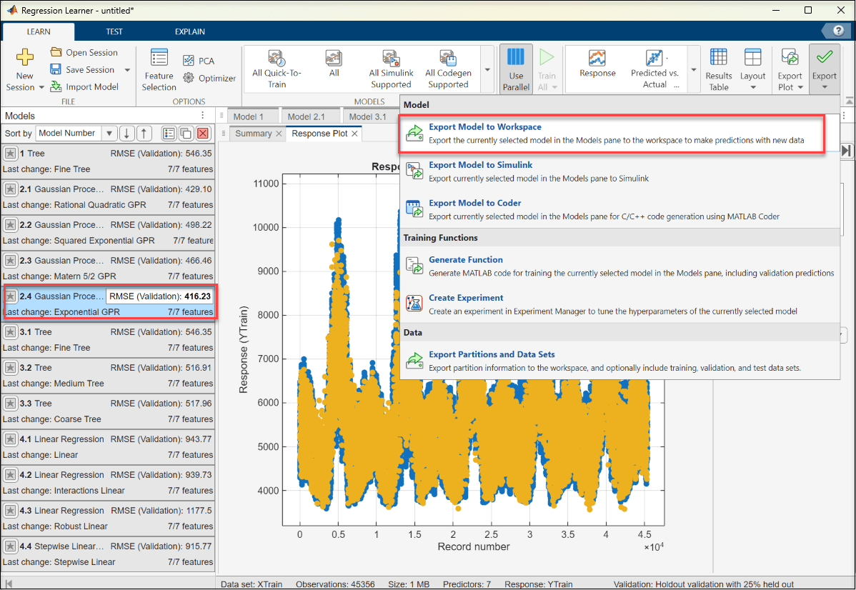
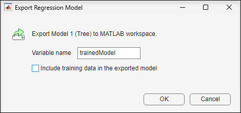
5. The exported model is saved in a variable named trainedModel in the current workspace. To exclude the training data and export a compact model, clear the check box in the Export Regression Model dialog box. You can still use the compact model for making predictions on new data.
Test Regression Model
To test the load prediction model, use the trained regression model to predict load values for the test data set. In this example, trainedModel is the variable name for the model exported from the Regression Learner app.
predictedLoad = trainedModel.predictFcn(XTest);
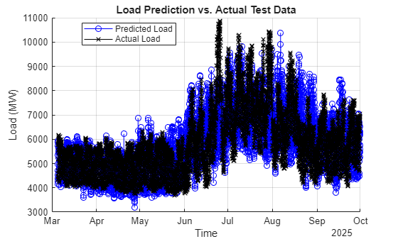
Compare the predicted values with the actual test data by plotting both.
figure;
hold on;
plot(timestampDataTest,predictedLoad,"-o","DisplayName","Predicted Load","Color","blue");
plot(timestampDataTest,YTest,"-x","DisplayName","Actual Load","Color","black");
hold off;

xlabel("Time");
ylabel("Load (MW)");
title("Load Prediction vs. Actual Test Data");
legend("show","Location","best");
grid on;
To evaluate the accuracy of the trained regression model, compute the root mean squared error (RMSE) between the predicted and target load values for the test data set. RMSE provides an absolute measure of prediction error, but it does not account for the scale of the data. To normalize the error and make it easier to interpret across different load ranges, calculate the coefficient of variation of RMSE (CV(RMSE)), which expresses RMSE as a percentage of the mean observed load.
residuals = YTest - predictedLoad;
TestRMSE = sqrt(mean(residuals.^2));
CVRMSE = (TestRMSE/mean(YTest))*100
CVRMSE = single

13.5747
Predict Future Load Requirement using Trained Model
To predict the future load requirement for a city, start by importing forecasted weather data. Weather data available online is often stored in CSV or XLSX format. Use the readtimetable function to import the data into MATLAB as a timetable.
This example uses a CSV file that contains weather data for October 1, 2025 — November 22, 2025. Use your own forecasted weather data in a similar format.
ForecastedWeatherData = readtimetable("WeatherData.csv")Display the first eight rows of the timetable.
head(ForecastedWeatherData)
          Time          AmbientAirTemperature    RelativeHumidity    AveragePrecipitation    WindFlowSpeed
    ________________    _____________________    ________________    ____________________    _____________

    10/01/2025 01:00              20                    60                    0                  14.6
    10/01/2025 02:00            18.6                    36                    0                  18.8
    10/01/2025 03:00            15.7                    47                    0                  14.1
    10/01/2025 04:00            14.8                    48                    0                    17
    10/01/2025 05:00            13.9                    50                    0                  16.3
    10/01/2025 06:00            13.3                    54                    0                  17.8
    10/01/2025 07:00            12.4                    58                    0                  14.5
    10/01/2025 08:00            13.5                    58                    0                  16.7
Once your data is in a similar format, follow these steps to forecast the load requirement using your trained model.
Extract Predictors
Extract weather-based predictors from the data set.
weatherData = ForecastedWeatherData{:,2:end};Extract time-based predictors from the data set.
timestampData = ForecastedWeatherData.Time;
monthData = month(timestampData);
hourData = hour(timestampData);
weekdayData = weekday(timestampData);
Combine Predictors
To obtain the final predictor data set, combine the weather-based and time-based data sets.
Xdata = [weatherData,monthData,hourData,weekdayData];
Predict and Visualize Load Requirement
Predict the future load requirement of a city using your predictor data set and trained regression model. Plot the forecasted load requirement.
forecastedLoadReq = trainedModel.predictFcn(Xdata);
plot(timestampData,forecastedLoadReq);
ylabel("Load Requirement (MW)")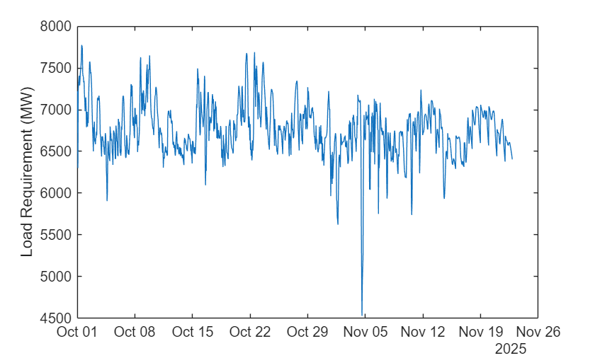
See Also
Functions
Apps
- Asset Framework Browser | Regression Learner (Statistics and Machine Learning Toolbox)
Topics
- Get Started with Accessing Data from AVEVA PI Asset Framework
- Train Regression Models in Regression Learner App (Statistics and Machine Learning Toolbox)