Profile and Optimize Generated GPU Code
This example shows how to profile and optimize generated GPU code using the GPU Performance Analyzer. You can use the GPU Performance Analyzer to generate code, profile the code, and detect performance bottlenecks. Use the performance diagnostics from the analyzer to modify the original MATLAB® function and improve performance of generated CUDA® code.
In this example, you identify issues in the GPU code generated for a fog rectification algorithm, trace between MATLAB and generated code, and optimize the code. For more information about fog rectification, see Generate GPU Code for Fog Rectification Algorithm.
Video Walkthrough
For a walkthrough of the example, play the video.
Verify GPU Environment
This example requires a GPU that can run CUDA code. To verify that the GPU is set up correctly, create a coder.gpuEnvConfig object and set the Quiet property to true. Use the coder.checkGpuInstall function.
envCfg = coder.gpuEnvConfig("host");
envCfg.Quiet = 1;
coder.checkGpuInstall(envCfg);
When the Quiet property of the coder.gpuEnvConfig object is true, the coder.checkGpuInstall function returns only warning or error messages. If the function does not generate an error, the GPU is set up for use with MATLAB.
Examine Fog Rectification Algorithm
In this example, you profile a fog rectification algorithm that removes fog and enhances image contrast to produce a defogged image. The diagram shows the steps for both these operations.
To remove fog from the image, the algorithm estimates the dark channel of the image, estimates and refines the airlight map, and restores the defogged image by subtracting the refined airlight map from the input image.
To enhance the contrast, the algorithm converts the restored image to grayscale and creates a normalized histogram of the intensity values. It then calculates the cumulative density function (CDF) of the intensity values, and uses contrast stretching to make the features stand out more clearly in the output image.
The MATLAB function fog_rectification_init implements the fog rectification algorithm.
type fog_rectification_init.mfunction [out] = fog_rectification_init(input) %#codegen
%
% Copyright 2025 The MathWorks, Inc.
coder.gpu.kernelfun;
% restoreOut is used to store the output of restoration
restoreOut = zeros(size(input),"double");
% Changing the precision level of input image to double
input = double(input)./255;
%% Dark channel Estimation from input
darkChannel = min(input,[],3);
% diff_im is used as input and output variable for anisotropic
% diffusion
diff_im = 0.9*darkChannel;
num_iter = 3;
% 2D convolution mask for Anisotropic diffusion
hN = [0.0625 0.1250 0.0625; 0.1250 0.2500 0.1250;
0.0625 0.1250 0.0625];
hN = double(hN);
%% Refine dark channel using Anisotropic diffusion.
for t = 1:num_iter
diff_im = conv2(diff_im,hN,"same");
end
%% Reduction with min
diff_im = min(darkChannel,diff_im);
diff_im = 0.6*diff_im ;
%% Parallel element-wise math to compute
% Restoration with inverse Koschmieder's law
factor = 1.0./(1.0-(diff_im));
restoreOut(:,:,1) = (input(:,:,1)-diff_im).*factor;
restoreOut(:,:,2) = (input(:,:,2)-diff_im).*factor;
restoreOut(:,:,3) = (input(:,:,3)-diff_im).*factor;
restoreOut = uint16(255.*restoreOut);
%%
% Stretching performs the histogram stretching of the image.
% im is the input color image and p is cdf limit.
% out is the contrast stretched image and cdf is the cumulative
% prob. density function and T is the stretching function.
% RGB to grayscale conversion
im_gray = im2gray(restoreOut);
[row,col] = size(im_gray);
% histogram calculation
count = zeros(256,1);
for i=1:numel(im_gray)
curr = im_gray(i)+1;
count(curr) = count(curr)+1;
end
prob = count/(row*col);
% cumulative Sum calculation
cdf = cumsum(prob(:));
% Utilize gpucoder.reduce to find less than particular probability.
% This is equal to "i1 = length(find(cdf <= (p/100)));", but is
% more GPU friendly.
% lessThanP is the preprocess function that returns 1 if the input
% value from cdf is less than the defined threshold and returns 0
% otherwise. gpucoder.reduce then sums up the returned values to get
% the final count.
i1 = gpucoder.reduce(cdf,@plus,"preprocess", @lessThanP);
i2 = 255 - gpucoder.reduce(cdf,@plus,"preprocess", @greaterThanP);
o1 = floor(255*.10);
o2 = floor(255*.90);
t1 = (o1/i1)*(0:i1);
t2 = (((o2-o1)/(i2-i1))*(i1+1:i2))-(((o2-o1)/(i2-i1))*i1)+o1;
t3 = (((255-o2)/(255-i2))*(i2+1:255))-(((255-o2)/(255-i2))*i2)+o2;
T = (floor([t1 t2 t3]));
restoreOut(restoreOut == 0) = 1;
u1 = (restoreOut(:,:,1));
u2 = (restoreOut(:,:,2));
u3 = (restoreOut(:,:,3));
% replacing the value from look up table
out1 = T(u1);
out2 = T(u2);
out3 = T(u3);
out = zeros([size(out1),3], "uint8");
out(:,:,1) = uint8(out1);
out(:,:,2) = uint8(out2);
out(:,:,3) = uint8(out3);
end
function out = lessThanP(input)
p = 5/100;
out = uint32(0);
if input <= p
out = uint32(1);
end
end
function out = greaterThanP(input)
p = 5/100;
out = uint32(0);
if input >= 1 - p
out = uint32(1);
end
end
Generate GPU Performance Analyzer Report
To analyze the performance of the generated code, first create a GPU code configuration object with the mex input argument.
cfg = coder.gpuConfig("mex");Run the GPU Performance Analyzer by specifying the function name, function inputs, and code configuration object to the gpuPerformanceAnalyzer function. The analyzer generates code, then executes the code twice. To exclude initialization overhead from the profiling data, it displays results from the second run by default.
designFileName = "fog_rectification_init";
inputImage = imread("foggyInput.png");
inputs  = {inputImage};

gpuPerformanceAnalyzer(designFileName,inputs, ...
    Config=cfg);
### Starting GPU code generation
Code generation successful: View report

### GPU code generation finished
### Starting application profiling
### Application profiling finished
### Starting profiling data processing
### Profiling data processing finished
### Showing profiling data

These numbers are representative. The actual values depend on your hardware setup. The profiling data in this example was generated using a machine with an 13th Gen Intel® Core™ i9-13900K CPU and an NVIDIA® GeForce® RTX 3080 Ti GPU.
Analyze Profiling Data
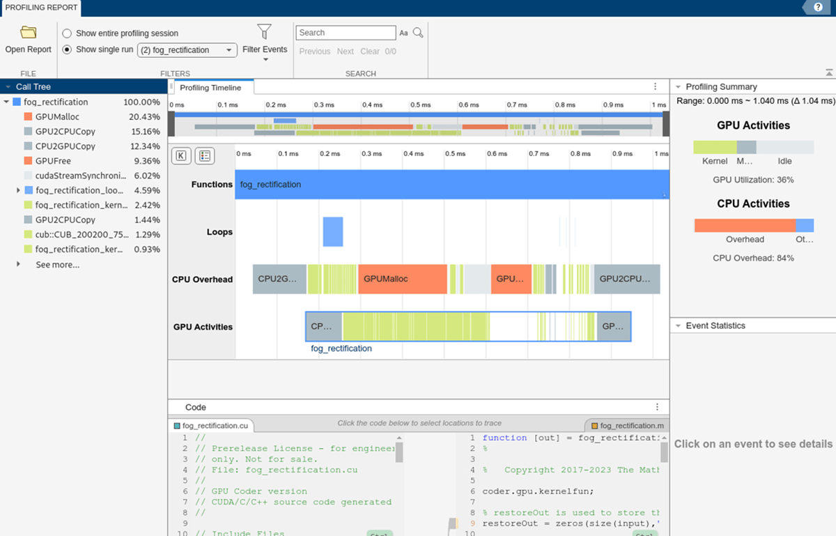
To view the CPU and GPU activities in the generated code, use the Profiling Timeline pane. In the Profiling Summary pane, the Range section shows the time range visible in the timeline. By default, the timeline shows the profiling data for the entire run. The generated code takes approximately 6.70 ms to execute. To improve the execution time, look for performance bottlenecks in the profiling data.
Analyze a Bottleneck Loop
During profiling, the GPU Performance Analyzer analyzes possible bottlenecks and flags them with a warning icon. In the Profiling Timeline pane, the analyzer flags the loop fog_rectification_loop_2.

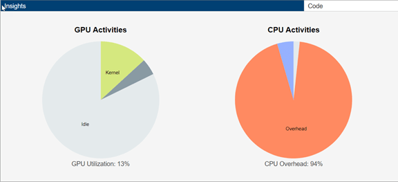
To examine the loop more closely, zoom in on it. In the timeline, hold Shift and click and drag your pointer over the event. You can also change the displayed time range using the mouse wheel. The Profiling Summary pane shows the CPU overhead and GPU utilization for the region in the timeline. After zooming in on fog_rectification_loop_2, the summary shows that the GPU utilization of the loop is 64%, which confirms that some of the execution time is spent on the CPU and not the GPU.
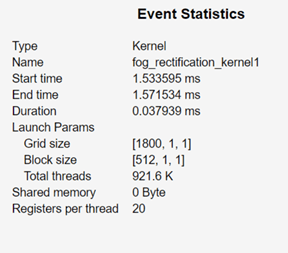
To get detailed statistics for the loop, in the Profiling Timeline pane, select fog_rectification_loop_2. The Event Statistics pane shows the loop executes for 4.38 ms and is idle for 3.66 ms. The loop spends approximately 0.72 ms executing on the CPU while the GPU is idle.
The generated code spends a significant amount of the application runtime executing the loop in serial on the CPU. To improve the performance, determine whether you can use the GPU to perform some of the computation.
Trace the CPU Loop
To determine how to improve the performance, trace the CPU loop to the source MATLAB code. In the Diagnostics pane, the GPU Performance Analyzer lists bottlenecks with code trace information, and, if possible, suggestions to optimize the bottleneck. View the diagnostic for fog_rectification_loop_2. To get more information about the loop, click Expand info. The Additional info section says that the variable count in the generated code causes a dependency that prevents GPU Coder from parallelizing the loop.

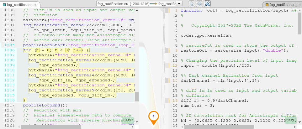
Click the link in the Relevant code section to view the generated code for fog_rectification_init_loop_2. The Code pane highlights the generated code for the loop in fog_rectification_init.cu.
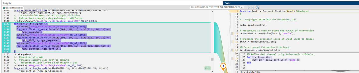
Point to the loop in fog_rectification_init.cu. The Code pane highlights the traced MATLAB code in fog_rectification_init.m.

To open the traced code in the MATLAB Editor, in the Code pane, click the line number. The traced code loops over the pixels in a grayscale image and calculates a histogram.
for i=1:numel(im_gray)
    curr = im_gray(i)+1;
    count(curr) = count(curr)+1;
end
The loop stores the histogram using a variable named count that has 256 elements. Each iteration increments the element of count that corresponds to the value of the pixel.
Rewrite the MATLAB Code
GPU Coder generates a CPU loop instead of a parallel GPU kernel because multiple iterations of the loop can access and modify the same memory location. If multiple threads execute the iterations of the loop in parallel, two threads can simultaneously update the same element of count, which causes a data race.
To generate a kernel, use the gpucoder.atomicAdd function to modify count. Using gpucoder.atomicAdd generates a kernel where each thread reads and modifies count atomically on the GPU.
for i=1:numel(im_gray)
    curr = im_gray(i)+1;
    count(curr) = gpucoder.atomicAdd(count(curr),1);
end
Save the new function as fog_rectification_atomic.
Profile the Updated MATLAB Function
To check whether the generated code for fog_rectification_atomic executes faster, generate and profile the code by using the gpuPerformanceAnalyzer function.
designFileName = "fog_rectification_atomic";
gpuPerformanceAnalyzer(designFileName,inputs,Config=cfg,OutFolder="newDesign");
### Starting GPU code generation
Code generation successful: View report

### GPU code generation finished
### Starting application profiling
### Application profiling finished
### Starting profiling data processing
### Profiling data processing finished
### Showing profiling data
In the Profiling Summary pane, the Range section shows the generated code for fog_rectification_atomic takes 4.97 ms to execute, which is approximately 1.35 times faster than the original entry-point function.