Multiprocessor Scheduling Using Simulated Annealing with a Custom Data Type
This example shows how to use simulated annealing to minimize a function using a custom data type. Here, simulated annealing is customized to solve the multiprocessor scheduling problem.
Multiprocessor Scheduling Problem
The multiprocessor scheduling problem consists of finding an optimal distribution of tasks on a set of processors. The number of processors and number of tasks are given. Time taken to complete a task by a processor is also provided as data. Each processor runs independently, but each can only run one job at a time. We call an assignment of all jobs to available processors a "schedule". The goal of the problem is to determine the shortest schedule for the given set of tasks.
First we determine how to express this problem in terms of a custom data type optimization problem that |simulannealbnd| function can solve. We come up with the following scheme: first, let each task be represented by an integer between 1 and the total number of tasks. Similarly, each processor is represented by an integer between 1 and the number of processors. Now we can store the amount of time a given job will take on a given processor in a matrix called "lengths". The amount of time "t" that the processor "i" takes to complete the task "j" will be stored in lengths(i,j).
We can represent a schedule in a similar manner. In a given schedule, the rows (integer between 1 to number of processors) will represent the processors and the columns (integer between 1 to number of tasks) will represent the tasks. For example, the schedule [1 2 3;4 5 0;6 0 0] would be tasks 1, 2, and 3 performed on processor 1, tasks 4 and 5 performed on processor 2, and task 6 performed on processor 3.
Here we define our number of tasks, number of processors, and lengths array. The different coefficients for the various rows represent the fact that different processors work with different speeds. We also define a "sampleSchedule" which will be our starting point input to simulannealbnd.
rng default % for reproducibility
numberOfProcessors = 11;
numberOfTasks = 40;
lengths = [10*rand(1,numberOfTasks);
    7*rand(1,numberOfTasks);
    2*rand(1,numberOfTasks);
    5*rand(1,numberOfTasks);
    3*rand(1,numberOfTasks);
    4*rand(1,numberOfTasks);
    1*rand(1,numberOfTasks);
    6*rand(1,numberOfTasks);
    4*rand(1,numberOfTasks);
    3*rand(1,numberOfTasks);
    1*rand(1,numberOfTasks)];

% Random distribution of task on processors (starting point)
sampleSchedule = zeros(numberOfProcessors,numberOfTasks);
for task = 1:numberOfTasks
    processorID = 1 + floor(rand*(numberOfProcessors));
    index = find(sampleSchedule(processorID,:)==0);
    sampleSchedule(processorID,index(1)) = task;
end
Simulated Annealing For a Custom Data Type
By default, the simulated annealing algorithm solves optimization problems assuming that the decision variables are double data types. Therefore, the annealing function for generating subsequent points assumes that the current point is a vector of type double. However, if the DataType option is set to "custom", the simulated annealing solver can also work on optimization problems involving arbitrary data types. You can use any valid MATLAB® data structure you like as decision variable. For example, if we want simulannealbnd to use "sampleSchedule" as decision variable, a custom data type can be specified using a matrix of integers. In addition to setting the DataType option to "custom" we also need to provide a custom annealing function via the AnnealingFcn option that can generate new points.
Custom Annealing Function
This section shows how to create and use the required custom annealing function. A trial point for the multiprocessor scheduling problem is a matrix of processor (rows) and tasks (columns) as discussed before. The custom annealing function for the multiprocessor scheduling problem will take a job schedule as input. The annealing function will then modify this schedule and return a new schedule that has been changed by an amount proportional to the temperature (as is customary with simulated annealing). The custom annealing function is mulprocpermute:
function schedule = mulprocpermute(optimValues,problemData)
% MULPROCPERMUTE Moves one random task to a different processor.
% NEWX = MULPROCPERMUTE(optimValues,problemData) generate a point based
% on the current point and the current temperature

% Copyright 2006 The MathWorks, Inc.

schedule = optimValues.x;
% This loop will generate a neighbor of "distance" equal to
% optimValues.temperature.  It does this by generating a neighbor to the
% current schedule, and then generating a neighbor to that neighbor, and so
% on until it has generated enough neighbors.
for i = 1:floor(max(optimValues.temperature))+1
    [nrows ncols] = size(schedule);
    schedule = neighbor(schedule, nrows, ncols);
end

%=====================================================%
function schedule = neighbor(schedule, nrows, ncols)
% NEIGHBOR generates a single neighbor to the given schedule.  It does so
% by moving one random task to a different processor.  The rest of the code
% is to ensure that the format of the schedule remains the same.

row1 = randinteger(1,1,nrows)+1;
col = randinteger(1,1,ncols)+1;
while schedule(row1, col)==0
    row1 = randinteger(1,1,nrows)+1;
    col = randinteger(1,1,ncols)+1;
end
row2 = randinteger(1,1,nrows)+1;
while row1==row2
    row2 = randinteger(1,1,nrows)+1;
end

for j = 1:ncols
    if schedule(row2,j)==0
        schedule(row2,j) = schedule(row1,col);
        break
    end
end

schedule(row1, col) = 0;
for j = col:ncols-1
    schedule(row1,j) = schedule(row1,j+1);
end
schedule(row1,ncols) = 0;
end
%=====================================================%
function out = randinteger(m,n,range)
%RANDINTEGER generate integer random numbers (m-by-n) in range

len_range = size(range,1) * size(range,2);
% If the IRANGE is specified as a scalar.
if len_range < 2
    if range < 0
        range = [range+1, 0];
    elseif range > 0
        range = [0, range-1];
    else
        range = [0, 0];    % Special case of zero range.
    end
end
% Make sure RANGE is ordered properly.
range = sort(range);

% Calculate the range the distance for the random number generator.
distance = range(2) - range(1);
% Generate the random numbers.
r = floor(rand(m, n) * (distance+1));

% Offset the numbers to the specified value.
out = ones(m,n)*range(1);
out = out + r;
end
end
Objective Function
We need an objective function for the multiprocessor scheduling problem. The objective function returns the total time required for a given schedule (which is the maximum of the times that each processor is spending on its tasks). As such, the objective function also needs the lengths matrix to be able to calculate the total times. We are going to attempt to minimize this total time. The objective function is mulprocfitness:
function timeToComplete = mulprocfitness(schedule, lengths)
%MULPROCFITNESS determines the "fitness" of the given schedule.
%  In other words, it tells us how long the given schedule will take using the
%  knowledge given by "lengths"

%   Copyright 2006 The MathWorks, Inc.

[nrows ncols] = size(schedule);
timeToComplete = zeros(1,nrows);
for i = 1:nrows
    timeToComplete(i) = 0;
    for j = 1:ncols
        if schedule(i,j)~=0
            timeToComplete(i) = timeToComplete(i)+lengths(i,schedule(i,j));
        else
            break
        end
    end
end
timeToComplete = max(timeToComplete);
end
simulannealbnd calls the objective function with just one argument x, but the objective function has two arguments: x and "lengths". Use an anonymous function to capture the values of the additional argument, the lengths matrix. Create a function handle ObjectiveFcn to an anonymous function that takes one input x, but calls mulprocfitness with x and lengths. The variable lengths has a value when the function handle FitnessFcn is created so these values are captured by the anonymous function.
lengths was defined earlier and so is in the workspace.
fitnessfcn = @(x) mulprocfitness(x,lengths);
Plot Function
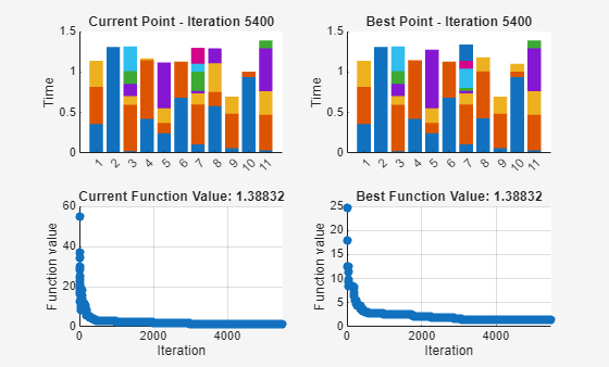
Add a custom plot function to plot the length of time that the tasks are taking on each processor. Each bar represents a processor, and the different colored chunks of each bar are the different tasks.
function stop = mulprocplot(~,optimvalues,flag,lengths)
%MULPROCPLOT PlotFcn used for SAMULTIPROCESSORDEMO
%   STOP = MULPROCPLOT(OPTIONS,OPTIMVALUES,FLAG) where OPTIMVALUES is a
%   structure with the following fields:
%              x: current point
%           fval: function value at x
%          bestx: best point found so far
%       bestfval: function value at bestx
%    temperature: current temperature
%      iteration: current iteration
%      funccount: number of function evaluations
%             t0: start time
%              k: annealing parameter "k"
%
%   FLAG: Current state in which PlotFcn is called. Possible values are:
%           init: initialization state
%           iter: iteration state
%           done: final state
%
%   STOP: A boolean to stop the algorithm.
%

%   Copyright 2006-2025 The MathWorks, Inc.

persistent thisTitle %#ok

stop = false;
switch flag
    case "init"
        set(gca,xlimmode="manual",zlimmode="manual", ...
            alimmode="manual")
        titleStr = sprintf("Current Point - Iteration %d", optimvalues.iteration);
        thisTitle = title(titleStr,interp="none");
        toplot = i_generatePlotData(optimvalues, lengths);
        ylabel("Time",interp="none");
        bar(toplot,"stacked",edgecolor="none");
        Xlength = size(toplot,1);
        set(gca,xlim=[0,1 + Xlength])
    case "iter"
        if ~rem(optimvalues.iteration, 100)
            toplot = i_generatePlotData(optimvalues, lengths);
            bar(toplot,"stacked",edgecolor="none");
            titleStr = sprintf("Current Point - Iteration %d", optimvalues.iteration);
            thisTitle = title(titleStr,interp="none");
        end
end

    function toplot = i_generatePlotData(optimvalues, lengths)

        schedule = optimvalues.x;
        nrows = size(schedule,1);
        % Remove zero columns (all processes are idle)
        maxlen = 0;
        for i = 1:nrows
            if max(nnz(schedule(i,:))) > maxlen
                maxlen = max(nnz(schedule(i,:)));
            end
        end
        schedule = schedule(:,1:maxlen);

        toplot = zeros(size(schedule));
        [nrows, ncols] = size(schedule);
        for i = 1:nrows
            for j = 1:ncols
                if schedule(i,j)==0 % idle process
                    toplot(i,j) = 0;
                else
                    toplot(i,j) = lengths(i,schedule(i,j));
                end
            end
        end
    end
end
Second Custom Plot Function
In simulated annealing, the current schedule is not necessarily the best schedule found so far. So create a second custom plot function that displays the best schedule that has been discovered so far.
function stop = mulprocplotbest(~,optimvalues,flag,lengths)
%MULPROCPLOTBEST PlotFcn used for SAMULTIPROCESSORDEMO
%   STOP = MULPROCPLOTBEST(OPTIONS,OPTIMVALUES,FLAG) where OPTIMVALUES is a
%   structure with the following fields:
%              x: current point
%           fval: function value at x
%          bestx: best point found so far
%       bestfval: function value at bestx
%    temperature: current temperature
%      iteration: current iteration
%      funccount: number of function evaluations
%             t0: start time
%              k: annealing parameter "k"
%
%   FLAG: Current state in which PlotFcn is called. Possible values are:
%           init: initialization state
%           iter: iteration state
%           done: final state
%
%   STOP: A boolean to stop the algorithm.
%

%   Copyright 2006-2025 The MathWorks, Inc.

persistent thisTitle %#ok

stop = false;
switch flag
    case "init"
        set(gca,xlimmode="manual",zlimmode="manual", ...
            alimmode="manual")
        titleStr = sprintf("Current Point - Iteration %d", optimvalues.iteration);
        thisTitle = title(titleStr,interp="none");
        toplot = i_generatePlotData(optimvalues, lengths);
        Xlength = size(toplot,1);
        ylabel("Time",interp="none");
        bar(toplot,"stacked",edgecolor="none");
        set(gca,xlim=[0,1 + Xlength])
    case "iter"
        if ~rem(optimvalues.iteration, 100)
            toplot = i_generatePlotData(optimvalues, lengths);
            bar(toplot,"stacked",edgecolor="none");
            titleStr = sprintf("Best Point - Iteration %d", optimvalues.iteration);
            thisTitle = title(titleStr,interp="none");
        end

end

    function toplot = i_generatePlotData(optimvalues, lengths)

        schedule = optimvalues.bestx;
        nrows = size(schedule,1);
        % Remove zero columns (all processes are idle)
        maxlen = 0;
        for i = 1:nrows
            if max(nnz(schedule(i,:))) > maxlen
                maxlen = max(nnz(schedule(i,:)));
            end
        end
        schedule = schedule(:,1:maxlen);

        toplot = zeros(size(schedule));
        [nrows, ncols] = size(schedule);
        for i = 1:nrows
            for j = 1:ncols
                if schedule(i,j)==0
                    toplot(i,j) = 0;
                else
                    toplot(i,j) = lengths(i,schedule(i,j));
                end
            end
        end
    end
end
Simulated Annealing Options Setup
Choose the custom annealing and plot functions, as well as change some of the default options. Set ReannealInterval to 800 because lower values for ReannealInterval seem to raise the temperature when the solver was beginning to make a lot of local progress. Decrease the StallIterLimit to 800 because the default value makes the solver too slow. Finally, set the DataType to "custom".
options = optimoptions(@simulannealbnd,DataType="custom", ...
    AnnealingFcn= @mulprocpermute,MaxStallIterations=800,ReannealInterval=800, ...
    PlotFcn={{@mulprocplot, lengths},{@mulprocplotbest, lengths},@saplotf,@saplotbestf});
Call Solver and Display Solution
The problem and options are complete. Call simulannealbnd to solve the problem.
schedule = simulannealbnd(fitnessfcn,sampleSchedule,[],[],options);
simulannealbnd stopped because the change in best function value is less than options.FunctionTolerance.
Remove the zero columns from the solution, which is where all processes are idle.
maxlen = 0;
for i = 1:size(schedule,1)
    if max(nnz(schedule(i,:)))>maxlen
        maxlen = max(nnz(schedule(i,:)));
    end
end
Display the resulting schedule.
schedule = schedule(:,1:maxlen)
schedule = 11×8

    22    34    32     0     0     0     0     0
     5     0     0     0     0     0     0     0
    19     6    12    11    39    35     0     0
     7    20     0     0     0     0     0     0
    30    15    10     3     0     0     0     0
    18    28     0     0     0     0     0     0
    31    33    29     4    21     9    25    40
    24    26    14     0     0     0     0     0
    13    16    23     0     0     0     0     0
    38    36     1     0     0     0     0     0
     8    27    37    17     2     0     0     0
      ⋮