Create Custom Plot Function

About Custom Plot Functions

If none of the plot functions that come with the software is suitable for the output you want to plot, you can write your own custom plot function, which the genetic algorithm calls at each generation to create the plot. This example shows how to create a plot function that displays the change in the best fitness value from the previous generation to the current generation.

Creating the Custom Plot Function

To create the plot function for this example, copy and paste the following code into a new file in the MATLAB^® Editor.

function state = gaplotchange(options, state, flag)
% GAPLOTCHANGE Plots the logarithmic change in the best score from the 
% previous generation.
%   
persistent last_best % Best score in the previous generation

if(strcmp(flag,'init')) % Set up the plot
    xlim([1,options.MaxGenerations]);
    axx = gca;
    axx.YScale = 'log';
    hold on;
    xlabel Generation
    title('Log Absolute Change in Best Fitness Value')
end

best = min(state.Score); % Best score in the current generation
if state.Generation == 0 % Set last_best to best.
    last_best = best;
else
	change = last_best - best; % Change in best score 
	last_best = best;
    if change > 0 % Plot only when the fitness improves
        plot(state.Generation,change,'xr');
    end
end

Save the file as gaplotchange.m in a folder on the MATLAB path.

Using the Custom Plot Function

To use the custom plot function, include it in the options.

rng(100) % For reproducibility
options = optimoptions('ga','PlotFcn',{@gaplotbestf,@gaplotchange});
[x,fval] = ga(@rastriginsfcn,2,[],[],[],[],[],[],[],options)

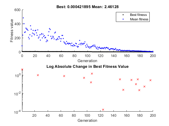
Optimization terminated: maximum number of generations exceeded.

x =

   -0.0003    0.0014


fval =

   4.2189e-04

The plot shows only changes that are greater than 0, which are improvements in best fitness. The logarithmic scale enables you to see small changes in the best fitness function that the upper plot does not reveal.

How the Plot Function Works

The plot function uses information contained in the following structures, which the genetic algorithm passes to the function as input arguments:

options — The current options settings
state — Information about the current generation
flag — Current status of the algorithm

The most important lines of the plot function are the following:

persistent last_best
Creates the persistent variable last_best—the best score in the previous generation. Persistent variables are preserved over multiple calls to the plot function.
xlim([1,options.MaxGenerations]);
axx = gca;
axx.YScale = 'log';
Sets up the plot before the algorithm starts. options.MaxGenerations is the maximum number of generations.
best = min(state.Score)
The field state.Score contains the scores of all individuals in the current population. The variable best is the minimum score. For a complete description of the fields of the structure state, see Structure of the Plot Functions.
change = last_best - best
The variable change is the best score at the previous generation minus the best score in the current generation.
if change > 0
Plot only if there is a change in the best fitness.
plot(state.Generation,change,'xr')
Plots the change at the current generation, whose number is contained in state.Generation.

The code for gaplotchange contains many of the same elements as the code for gaplotbestf, the function that creates the best fitness plot.