Track Targets Using Asynchronous Bistatic Radars

Since R2025a

This example builds upon the Tracking Using Bistatic Range Detections example and shows how to configure a multi-sensor multi-target tracker to track targets using asynchronous bistatic radars that report range and angles. Bistatic sensors are advantageous because the emitter part and the receiver part of the sensor are not collocated, which makes the receivers less detectable. Additionally, they allows many receivers to work with a single emitter. Therefore, bistatic sensors are becoming more common in various applications where it is beneficial to hide the receivers or reduce the amount of energy they consume.

Introduction

A bistatic radar is a pair of a bistatic emitter and a bistatic receiver. The geometry of a bistatic system is depicted in the figure below. The emitter emits signals that propagate towards the target and the receiver. The receiver receives both signals. One signal reflects off the target and propagates to the receiver along the path forming the upper sides of the triangle ($$R_E+R_R$$). The direct path from the emitter to the receiver propagates the length between the two, denoted by L. The relative bistatic range is given by:

$${\mathit{R}}_{\mathrm{Bistatic}}={\mathit{R}}_{\mathit{E}}+{\mathit{R}}_{\mathit{R}}-\mathit{L}$$

where $$R_E$$ is the range from the emitter to the target, $$R_R$$ is the range from the target to the receiver, and $$L$$, known also as the direct-path or baseline, is the range from the emitter to the receiver. The distance L is assumed to be known. Therefore, the emitter and receiver serve as focal points to an ellipse defined by the distance ${\mathit{R}}_{\mathit{E}}+{\mathit{R}}_{\mathit{R}}$. The target is, therefore, somewhere along the ellipse. If, in addition to the bistatic range, the receiver measures the angle to the target, as denoted by the angle between L and $$R_R$$, there is a unique point on the ellipse that defines the target position. This geometry scales to three dimensions by defining an ellipsoid and two angles.

In the Tracking Using Bistatic Range Detections example, it was necessary to use a static data fuser that performed data association between multiple measurements in a multi-target scenario in the presence of false alarms. The static data fusion algorithm assumed that the sensors reported measurements at the same time, in other words, that the sensors were synchronous.

In many applications, it is difficult or undesirable to synchronize sensors. Some bistatic receivers can report azimuth angle, and even elevation angle to the target, in addition to the bistatic range. This allows for Gaussian position estimates of targets based on just one measurement and alleviates the need for sensor synchronization. Reported measurements can be associated and fused using a multi-object tracker, even when the sensors are asynchronous and report at different times. In this example, you track multiple targets with such bistatic sensors.

Create Scenario

In this section, create a trackingScenario similar to the one used in the Tracking Using Bistatic Range Detections example. However, to show the asynchronous nature of the bistatic receivers, each receiver has a different update rate.

rng(2050); % For repeatable results
scenario = trackingScenario;
scenario.StopTime = 30.01;    % sec

Create an omnidirectional radar emitter using the radarEmitter object with the same parameters as those used in the Tracking Using Bistatic Range Detections example. Mount the emitter on a stationary platform at the scenario origin.

emitterIdx = 1; % Emitter is added as first platform in scene
emitter = radarEmitter(emitterIdx,'No scanning', ...
    'UpdateRate', 6, ...            % Emitter emits 6 times per second
    'FieldOfView',[360 180], ...    % [az el] deg
    'CenterFrequency', 300e6, ...   % Hz
    'Bandwidth', 30e6, ...          % Hz
    'WaveformType', 1);             % Use 1 for an LFM-like waveform 
emitterPlat = platform(scenario,'Trajectory',kinematicTrajectory('Position',[0 0 0],...
    'Velocity',[0 0 0]));
emitterPlat.Emitters = {emitter};

Next, create four receivers with different update rates and define the scenario rate to be the common denominator of all of them. This creates a situation where, at every scenario update, there are between zero and four receivers reporting. For example, at time 1/6 second, none of the receivers report, at time 1/3 seconds, only the second receiver reports, and at time 1 seconds, the first three receivers report.

numReceivers = 4;
updateRates = [2 3 0.5 1];
scenario.UpdateRate = 6;  

Create a receiver using the fusionRadarSensor object. For simplicity and to ensure that the receivers cover both the emitter and the targets at the same time, assume that the receivers are not scanning and are also omnidirectional.

receiver = fusionRadarSensor(1,'No scanning', ...                
    'FieldOfView',[360 180], ...    % [az el] deg 
    'DetectionMode','Bistatic', ... % Bistatic detection mode
    'CenterFrequency', 300e6, ...   % Hz
    'Bandwidth', 30e6, ...          % Hz
    'WaveformTypes', 1,...          % Use 1 for an LFM-like waveform 
    'HasINS',true,...               % Has INS to enable tracking in scenario 
    'AzimuthResolution',5,...       
    'HasElevation',true,...         % Enable elevation to set elevation resolution
    'HasRangeRate',true,...         % Enable range-rate measurement
    'FalseAlarmRate',1e-7,...       % Reduce false alarm rate to counter the full scenario coverage
    'RangeLimits',[0 10000],...     % Reduce range limits to reduce overall number of false alarms
    'Sensitivity',-35,...           % Reduce sensitivity due to short ranges
    'ElevationResolution',10);

receivers = cell(1,numReceivers);
for iD = 1:numReceivers
    receivers{iD} = clone(receiver); % Clone the bistatic receiver.
    receivers{iD}.SensorIndex = iD;  % Provide a unique sensor index to each receiver.
    receivers{iD}.UpdateRate = updateRates(iD); % Each sensor has a different update rate.
end

Mount the receivers on stationary platforms positioned at random places around the origin. You can add velocity to the receiver platforms if needed by providing a nonzero velocity vector in the code below.

r = 2000;                                          % Range, m
theta = linspace(0,pi,numReceivers);               % Theta, rad
xSen = r*cos(theta) + 100*randn(1,numReceivers);   % m 
ySen = r*sin(theta) + 100*randn(1,numReceivers);   % m
zSen = -1000*rand(1,numReceivers);                 % m
sensorPlats = cell(1,numReceivers);
for iD = 1:numReceivers
    sensorPlats{iD} = platform(scenario,...
        'Trajectory',kinematicTrajectory('Position',[xSen(iD) ySen(iD) zSen(iD)],...
        'Velocity',[0 0 0]));
    sensorPlats{iD}.Signatures{1} = rcsSignature(Pattern=-100); % Avoid detections from sensor platforms
    sensorPlats{iD}.Sensors = receivers{iD};
end

Finally, define four targets that move along a straight line with constant speed around the origin. The target initial positions and velocities are random.

numTargets = 4;
r = abs(2000*randn(1,numTargets));                % Random ranges, m
theta = linspace(0,numTargets*pi/4,numTargets);   % Angular position, rad
xTgt = r.*cos(theta) + 100*randn(1,numTargets);   % x position, m
yTgt = -r.*sin(theta) + 100*randn(1,numTargets);  % y position, m
zTgt = -1000*ones(1,numTargets);                  % z position, m

for iD = 1:numTargets
    thisPlat = platform(scenario,...
        'Trajectory',kinematicTrajectory('Position',[xTgt(iD) yTgt(iD) zTgt(iD)],...
        'Velocity',[10*randn 10*randn 5*randn]));
end

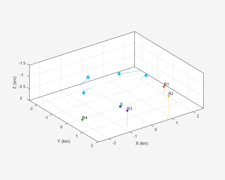
Use the initializeTheaterPlot function attached to this example to visualize the scenario and create the theaterPlot object, tp.

tp = initializeTheaterPlot(scenario);

Understand Track Initialization using Bistatic Radar Detection

This section describes how to use a bistatic radar detection to initialize a Gaussian track. The code below depicts the first bistatic measurement reported by the first receiver, which is a measurement of the last platform in the scenario. The mesh depicts the ellipsoid created by the total distance from the emitter to the target and from the target to receiver R1. The red patch depicts the azimuth and elevation angle measurements, including uncertainty. The intersection of the mesh and the ellipsoid represents the measured position.

measurement = struct(Azimuth=-175.6312,Elevation=-11.709,Range=3575.5,RangeRate=-9.6687, ...
    AzimuthAccuracy=0.8476,ElevationAccuracy=1.6953,RangeAccuracy=13.0697,RangeRateAccuracy=1.307);
visualizeOneDetection(measurement,scenario,tp,Simplify=false);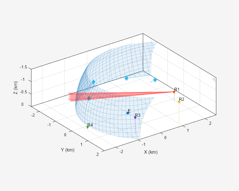

Since the emitter and receiver positions are known, it is possible to solve for the intersection point between the ellipsoid and the measurement. The solution provides the estimated position in Cartesian coordinates, which allows you to initialize a Gaussian track. In the next section, you create a bistatic radar sensor specification, which uses this computation to initialize a tracks.

To simplify the visualization for the multi-target case, the line shown in the figure below depicts the same geometry as shown in the the previous figure, but is less cluttered.

estimatedTgtPosition = [-1592 -75.45 -1114.2]; % The estimated position from this measurement
visualizeOneDetection(estimatedTgtPosition,scenario,tp,Simplify=true);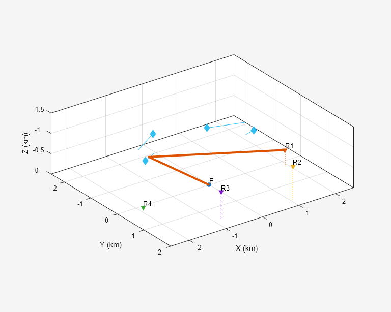

Define a Multi-Target Bistatic Radar Tracker

To track multiple targets using the bistatic radar measurements, create a bistatic sensor specification for each pair of emitter and receiver. First, create one bistatic radar specification and configure the common parameters that impact its data format like measurement mode, stationary flags, and measurement flags. Use the trackerSensorSpec function to create the bistatic radar specification and use tab-completion to define the aerospace radar as bistatic.

spec = trackerSensorSpec("aerospace","radar","bistatic");
spec.MeasurementMode = "range-angle";  % fusionRadarSensor bistatic mode reports angles
spec.IsReceiverStationary = true;      % Receiver is stationary in this example
spec.IsEmitterStationary = true;       % Emitter is stationary in this example
spec.MaxNumLooksPerUpdate = 1;         % One look per tracker update
spec.MaxNumMeasurementsPerUpdate = 10; % Number of true and false measurements per update

In a simulated scenario such as the one in this example, you can use the emitter and receiver parameters to create the bistatic sensor specifications as shown in the next code block. In the case of data recorded in the real world, use the information from the emitter and receiver datasheets to define the bistatic radar specifications.

sensorSpecs = repmat({spec},1,numReceivers);
for iD = 1:numReceivers
    spec = sensorSpecs{iD};
    receiver = sensorPlats{iD}.Sensors{1};
    spec.HasElevation = receiver.HasElevation; % Match the receiver elevation flag
    spec.HasRangeRate = receiver.HasRangeRate; % Match the receiver range rate flag
    spec.EmitterPlatformPosition = emitterPlat.Position;
    spec.EmitterPlatformOrientation = rotmat(quaternion(emitterPlat.Orientation,'eulerd','ZXY','frame'),"frame");
    spec.EmitterMountingLocation = emitter.MountingLocation;
    spec.EmitterMountingAngles = emitter.MountingAngles;
    spec.EmitterFieldOfView = emitter.FieldOfView;
    spec.ReceiverPlatformPosition = sensorPlats{iD}.Position;
    spec.ReceiverPlatformOrientation = rotmat(quaternion(sensorPlats{iD}.Orientation,'eulerd','ZXY','frame'),"frame");
    spec.ReceiverMountingLocation = receiver.MountingLocation;
    spec.ReceiverMountingAngles = receiver.MountingAngles;
    spec.ReceiverFieldOfView = receiver.FieldOfView;
    spec.ReceiverRangeLimits = receiver.RangeLimits;
    spec.ReceiverRangeRateLimits = receiver.RangeRateLimits;
    spec.AzimuthResolution = receiver.AzimuthResolution;
    spec.ElevationResolution = receiver.ElevationResolution;
    spec.RangeResolution = receiver.RangeResolution;
    spec.RangeRateResolution = receiver.RangeRateResolution;
    spec.DetectionProbability = receiver.DetectionProbability;
    spec.FalseAlarmRate = receiver.FalseAlarmRate;
    sensorSpecs{iD} = spec;
end

Next, use the trackerTargetSpec function to define the tracker target specification that is appropriate in this case. Choose the aerospace helicopter specification for aerial targets that follow a relatively slow constant velocity model.

tgtspec = trackerTargetSpec("aerospace","aircraft","helicopter");

Finally, use the multiSensorTargetTracker function to specify a JIPDATracker that tracks helicopter targets using the bistatic sensor specifications you defined earlier. As the sensor specifications assume a very low false alarm rate, increase the confirmation existence probability threshold to prevent the tracker from confirming false tracks on the first detection.

tracker = multiSensorTargetTracker(tgtspec,sensorSpecs,"jipda");
tracker.ConfirmationExistenceProbability = 0.98;
tracker.MaxMahalanobisDistance = 10;

Prepare the Sensor Data

In this section, prepare the sensor data to match the data needed by the bistatic sensor specifications. If you have recorded data from a real sensor, you would load it and map the data elements to the format that the specification defines.

First, review the expected data for each specification using the dataFormat object function. For brevity, show only one of the specifications.

expectedFormat = dataFormat(sensorSpecs{1});
disp(expectedFormat);

         ReceiverLookTime: 0
      ReceiverLookAzimuth: 0
    ReceiverLookElevation: 0
       EmitterLookAzimuth: 0
     EmitterLookElevation: 0
            DetectionTime: [0 0 0 0 0 0 0 0 0 0]
                  Azimuth: [0 0 0 0 0 0 0 0 0 0]
                Elevation: [0 0 0 0 0 0 0 0 0 0]
                    Range: [0 0 0 0 0 0 0 0 0 0]
                RangeRate: [0 0 0 0 0 0 0 0 0 0]
          AzimuthAccuracy: [0 0 0 0 0 0 0 0 0 0]
        ElevationAccuracy: [0 0 0 0 0 0 0 0 0 0]
            RangeAccuracy: [0 0 0 0 0 0 0 0 0 0]
        RangeRateAccuracy: [0 0 0 0 0 0 0 0 0 0]

Use the recordBistaticData helper function attached to this example to create the bistatic data in a format that matches the data format.

data = recordBistaticData(scenario,sensorSpecs);

To verify that the recorded data format matches the expected format, you can check that all the expected fields are provided.

expectedFieldNames = fieldnames(expectedFormat);
providedFieldNames = fieldnames(data{1});
containsExpectedFields = isempty(setdiff(expectedFieldNames,providedFieldNames))

containsExpectedFields = logical
   1

Run the Scenario

The following code runs the scenario. In case you ran the scenario earlier, you must first restart the scenario, reset the tracker, and preallocate the memory before running the while-loop. To select data from each time interval before passing it to the tracker, use the selectData helper function provided with this example. To visualize the scenario, detections, and tracks, use the updateTheaterPlot helper function also provided with this example.

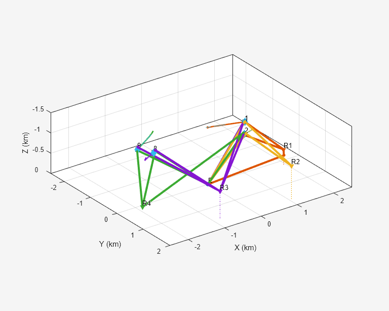
restart(scenario);
prevTimeStamp = 0;
reset(tracker);
ospa = trackOSPAMetric(Metric="OSPA(2)",Distance="posabserr",WindowLength=12,CutoffDistance=100);
ospaValues = zeros(1,floor(scenario.StopTime*scenario.UpdateRate));
resetTheaterPlot(tp);
i = 0;
while advance(scenario)
    poses = platformPoses(scenario);
    currentData = selectData(data, prevTimeStamp, scenario.SimulationTime);
    tracks = tracker(currentData{:});
    i = i + 1;
    ospaValues(i) = ospa(tracks,poses(6:end));
    
    updateTheaterPlot(tp,poses,tracks,sensorSpecs,currentData);

    prevTimeStamp = scenario.SimulationTime;
end

Analyze the Tracking Results

The visualization above showed that the tracker quickly established tracks on the targets and kept these tracks stable throughout the scenario. Additionally, there are no noticeable false tracks.

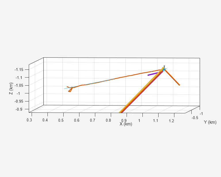
Zoom in on Track 1 to observe the tracking accuracy. This view shows how the track follows accurately the truth in light blue.

tp.XLimits = [280 1270];
tp.YLimits = [-1010 -120];
tp.ZLimits = [-1180 -880];
view([6 3]);

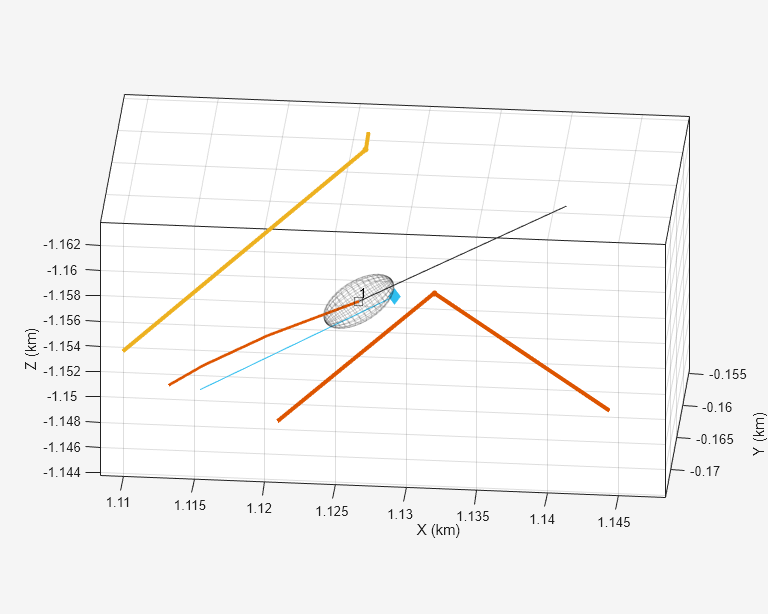
Zooming in even further on the last track update. At this zoom level, you can observe how the track 1-sigma uncertainty almost encircles the truth position with less than 10 meters distance from the true position. Meanwhile, the detections, indicated by the intersecting lines and point, are much farther away from it.

pos = poses(7,:).Position;
tp.XLimits = pos(1) + [-20 20];
tp.YLimits = pos(2) + [-10 10];
tp.ZLimits = pos(3) + [-10 10];
view([-5 -27]);

To quantitatively assess the tracking quality, use the Optimal Sub-Pattern Assignment (OSPA) metric that compares tracks and ground truth. As a reminder, the OSPA(2) metric adds a penalty for every missed truth, false track, track switch, or kinematic errors; therefore, lower OSPA values indicate better tracking quality.

ax = axes(figure);
plot(ax,(1:i)/scenario.UpdateRate,ospaValues);
xlabel("Time [sec]");
ylabel("OSPA(2)");
title("OSPA Values vs. Time")

As the plot shows, the OSPA(2) metric rapidly decreases, indicating quick track establishment, and remains low for the duration of the scenario. This result indicates good and consistent tracking of all the targets without false alarms.

Summary

This example showed how to use the task-oriented tracker to track multiple targets using asynchronous bistatic radars that report range and angles. The example showed how to define a scenario, configure the bistatic radar sensor specifications, and use the tracker.

Having bistatic radars that report both range and angles instead of range-only measurements allows the tracker to initialize Gaussian tracks based on a single bistatic measurement. Thus, there is no longer a need for static data fusion, which was needed to obtain Gaussian tracks in the case of range-only measurements, and the sensors could report their measurements asynchronously.

Supporting Functions

visualizeOneDetection - A helper to visualize one bistatic detection, including its ellipse and angle

function visualizeOneDetection(measurement,scenario,tp,options)
arguments
    measurement
    scenario (1,1) trackingScenario
    tp (1,1) theaterPlot
    options.Simplify (1,1) logical = false;
end

exPos = scenario.Platforms{1}.Position(:); % Emitter position
rxPos = scenario.Platforms{2}.Position(:); % Receiver 1 position

if options.Simplify
    hSurf = findobj(tp.Parent,Tag="EllipsoidSurf");
    if ishghandle(hSurf)
        delete(hSurf);
    end
    hPatch = findobj(tp.Parent,Tag="MeasurementPatch");
    if ishghandle(hPatch)
        delete(hPatch);
    end
    linePositions = [exPos';measurement;rxPos'];
    hLine = findobj(tp.Parent,Tag="DetLines2");
    hLine.XData = linePositions(:,1);
    hLine.YData = linePositions(:,2);
    hLine.ZData = linePositions(:,3);
    drawnow
    return
end

relVec = rxPos - exPos;

L = norm(rxPos - exPos);
R = measurement.Range + L;
a = R/2;
e = L/(2*a);
center = (rxPos + exPos)/2;
b = a*sqrt(1 - e^2);

phi = linspace(-180,180,100);
theta = linspace(-90,90,50);
[Theta,Phi] = meshgrid(theta,phi);

thisX = a*cosd(Phi).*cosd(Theta);
thisY = b*sind(Phi).*cosd(Theta);
thisZ = b.*sind(Theta);

u1 = relVec/norm(relVec);
u2 = [-u1(2);u1(1);0];
u2 = u2/norm(u2);
u3 = cross(u1,u2);
rot = [u1 u2 u3];
X = rot(1,1)*thisX + rot(1,2)*thisY + rot(1,3)*thisZ + center(1);
Y = rot(2,1)*thisX + rot(2,2)*thisY + rot(2,3)*thisZ + center(2);
Z = rot(3,1)*thisX + rot(3,2)*thisY + rot(3,3)*thisZ + center(3);
thisClr = lines(1);
hold on;
surf(tp.Parent,X,Y,Z,'FaceColor',thisClr,'Marker','none','FaceAlpha',0.1,'EdgeAlpha',0.3,'EdgeColor',thisClr,Tag="EllipsoidSurf");

% Add a patch showing the detection + uncertainty reported by the receiver
Phi = measurement.Azimuth + measurement.AzimuthAccuracy.*[1;1;-1;-1];
Theta = measurement.Elevation + measurement.ElevationAccuracy.*[1;-1;-1;1];
X = rxPos(1)+[0;R*cosd(Phi).*cosd(Theta)];
Y = rxPos(2)+[0;R*sind(Phi).*cosd(Theta)];
Z = rxPos(3)+[0;R*sind(Theta)];
vertices = [X Y Z];
faces = [1 2 3 1;1 2 4 1;1 2 5 1;1 3 4 1;1 3 5 1;1 4 5 1];
patch(tp.Parent,Faces=faces,Vertices=vertices,FaceColor=[1 0 0],FaceAlpha=0.1,EdgeAlpha=0.3,EdgeColor=[1 0 0],Tag="MeasurementPatch");

hLine = findobj(tp.Parent,Tag="DetLines2");
hLine.XData = NaN;
hLine.YData = NaN;
hLine.ZData = NaN;
end

initializeTheaterPlot - A helper function to initialize a theaterPlot object based on the example scenario.

function tp = initializeTheaterPlot(scenario)
f = figure(Units="normalized",Position=[0.2 0.2 0.6 0.6],Visible="off");
ax = axes(f);
ax.ZDir = "reverse";  
tp = theaterPlot(Parent=ax,AxesUnits=["km" "km" "km"],XLimits=[-2500 2500], ...
    YLimits=[-2500 2000],ZLimits=[-1500 0]);

restart(scenario); % In case scenario is not restarted yet
clrs = lines(numel(scenario.Platforms));
containsEmitters = cellfun(@(p) ~isempty(p.Emitters), scenario.Platforms);
numEmitters = nnz(containsEmitters);
emitterInds = find(containsEmitters);
for i = 1:numEmitters
    emitterPlotter = platformPlotter(tp,DisplayName="Emitter"+emitterInds(i), ...
        Marker="o",MarkerEdgeColor=clrs(i,:),MarkerFaceColor=clrs(i,:),MarkerSize=6);
    plotPlatform(emitterPlotter,scenario.Platforms{emitterInds(i)}.Position,"E");
end

containsSensors = cellfun(@(p) ~isempty(p.Sensors), scenario.Platforms);
numSensors = nnz(containsSensors);
sensorInds = find(containsSensors);
hold on
for i = 1:numSensors
    ci = sensorInds(i);
    position = scenario.Platforms{sensorInds(i)}.Position;
    sensorPlotter = platformPlotter(tp,DisplayName="Sensor"+ci, ...
        Marker="v",MarkerEdgeColor=clrs(ci,:),MarkerFaceColor=clrs(ci,:),MarkerSize=6);
    plotPlatform(sensorPlotter,position,"R"+i);
    detectionPlotter(tp,DisplayName="Detections"+ci,Tag="Detections"+ci, ...
        Marker="o",MarkerEdgeColor=clrs(ci,:),MarkerFaceColor=clrs(ci,:),MarkerSize=4);
    plot3(repmat(position(1),2,1),repmat(position(2),2,1),[position(3);0],Color=clrs(ci,:),LineStyle=":");
    plot3(tp.Parent,NaN,NaN,NaN,Color=clrs(ci,:), ...
        LineWidth=3,Marker=".",MarkerSize=5,Tag="DetLines"+ci);
end
hold off

platInds = find(~containsSensors & ~containsEmitters);
numPlatforms = numel(platInds);
clr = clrs(ci+1,:);
tgtPlotter = platformPlotter(tp,DisplayName="Targets",Marker="d", ...
    MarkerEdgeColor=clr,MarkerFaceColor=clr,MarkerSize=8);
poses = platformPoses(scenario);
tgtPoses = poses(platInds);
tgtPositions = vertcat(tgtPoses.Position);
tgtVelocities = vertcat(tgtPoses.Velocity);
plotPlatform(tgtPlotter,tgtPositions);
hold on;
for i = 1:numPlatforms    
    xyz = [tgtPositions(i,:);tgtPositions(i,:)+tgtVelocities(i,:)*scenario.StopTime];
    plot3(xyz(:,1),xyz(:,2),xyz(:,3),Color=clr);
end

trackPlotter(tp,DisplayName="Tracks",Marker="s",MarkerSize=8, ...
    ConnectHistory="on",ColorizeHistory="on");
grid(ax,'on')
set(ax,'YDir','reverse','ZDir','reverse');
view(ax,-36,26);
legend off
f.Visible = "on";
end

recordBistaticData - A helper function to record bistatic sensor data from the scenario using the data format defined by the sensor specifications.

function data = recordBistaticData(scenario, sensorSpecs)
restart(scenario);

% Reproducible geometry
rng(2021);

detlog = {};
i = 0;
while advance(scenario)
    % Emit radar emissions
    [txEmiss,configs] = emit(scenario);

    % Propagate the radar emissions
    prEmiss = propagate(scenario, txEmiss, HasOcclusion = false);

    % Create radar detections
    i = i + 1;
    detections = detect(scenario, prEmiss, configs);
    if scenario.SimulationTime > 0 % Avoid the t=0 synchronization
        detlog = [detlog;detections]; %#ok<AGROW>
    end
end
data = formatBistaticDetections(detlog,sensorSpecs);
end

formatBistaticDetections - A helper function to convert bistatic detections log to the data format defined by the sensor specifications.

function data=formatBistaticDetections(detlog,specs)
if iscell(detlog{1})
    detlog = vertcat(detlog{:});
end
ind = cellfun(@(d) d.SensorIndex, detlog);
numSpecs = numel(specs);
data = cell(1,numSpecs);
for id = 1:numSpecs
    thisSensor = (ind==id);
    data{id} = formatDetectionsOneSpec(detlog(thisSensor),specs{id});
end

    function data = formatDetectionsOneSpec(detlog,spec)
        detlog = [detlog{:}];
        data = dataFormat(spec);
        data.ReceiverLookTime = unique(arrayfun(@(d) d.Time, detlog));
        numLooks = numel(data.ReceiverLookTime);
        data.ReceiverLookAzimuth = zeros(1,numLooks); % Receiver is omnidirectional
        data.ReceiverLookElevation = zeros(1,numLooks); % Receiver is omnidirectional
        data.EmitterLookAzimuth = zeros(1,numLooks); % Emitter is omnidirectional
        data.EmitterLookElevation = zeros(1,numLooks); % Emitter is omnidirectional
        data.DetectionTime = arrayfun(@(d) d.Time, detlog);
        data.Azimuth = arrayfun(@(d) d.Measurement(1), detlog);
        data.Elevation = arrayfun(@(d) d.Measurement(2), detlog);
        data.Range = arrayfun(@(d) d.Measurement(3), detlog);
        data.RangeRate = arrayfun(@(d) d.Measurement(4), detlog);
        data.AzimuthAccuracy = sqrt(arrayfun(@(d) d.MeasurementNoise(1,1), detlog));
        data.ElevationAccuracy = sqrt(arrayfun(@(d) d.MeasurementNoise(2,2), detlog));
        data.RangeAccuracy = sqrt(arrayfun(@(d) d.MeasurementNoise(3,3), detlog));
        data.RangeRateAccuracy = sqrt(arrayfun(@(d) d.MeasurementNoise(4,4), detlog));
        data.TargetIndex = arrayfun(@(d) d.ObjectAttributes{1}.TargetIndex, detlog);
    end
end

selectData - A helper function to select bistatic sensor data obtained between the previous and current timestamps. This data is passed to the tracker at each tracker update.

function currentData = selectData(data, prevTime, currentTime)
numSensors = numel(data);
currentData = cell(1,numSensors);
for i = 1:numSensors
    thisData = data{i};
    lookIndices = thisData.ReceiverLookTime > prevTime & thisData.ReceiverLookTime <= currentTime;
    thisData.ReceiverLookTime = thisData.ReceiverLookTime(lookIndices);
    thisData.ReceiverLookAzimuth = thisData.ReceiverLookAzimuth(lookIndices);
    thisData.ReceiverLookElevation = thisData.ReceiverLookElevation(lookIndices);
    thisData.EmitterLookAzimuth = thisData.EmitterLookAzimuth(lookIndices);
    thisData.EmitterLookElevation = thisData.EmitterLookElevation(lookIndices);
    detIndices = thisData.DetectionTime > prevTime & thisData.DetectionTime <= currentTime;
    thisData.DetectionTime = thisData.DetectionTime(detIndices);
    thisData.Azimuth = thisData.Azimuth(detIndices);
    thisData.Elevation = thisData.Elevation(detIndices);
    thisData.Range = thisData.Range(detIndices);
    thisData.RangeRate = thisData.RangeRate(detIndices);
    thisData.AzimuthAccuracy = thisData.AzimuthAccuracy(detIndices);
    thisData.ElevationAccuracy = thisData.ElevationAccuracy(detIndices);
    thisData.RangeAccuracy = thisData.RangeAccuracy(detIndices);
    thisData.RangeRateAccuracy = thisData.RangeRateAccuracy(detIndices);
    currentData{i} = thisData;
end
end

updateTheaterPlot - A helper function to update the truth, measurements, and tracks on the theater plot.

function updateTheaterPlot(tp,poses,tracks,sensorSpecs,currentData)
pp = findPlotter(tp,DisplayName="Targets");
trp = findPlotter(tp,DisplayName="Tracks");

% Update platform positions
tgtPositions = vertcat(poses(6:end).Position);
plotPlatform(pp,tgtPositions);

% Update tracks
trackIDs = [tracks.TrackID];
[pos,cov] = getTrackPositions(tracks,"constvel");
vel = getTrackVelocities(tracks,"constvel");
plotTrack(trp,pos,vel,cov,string(trackIDs),trackIDs);

% Plot bistatic sensor data using the sensor specifications
numSensors = numel(sensorSpecs);
for i = 1:numSensors
    thisSpec = sensorSpecs{i};
    thisData = currentData{i};
    measurement = [thisData.Azimuth;thisData.Elevation;thisData.Range;thisData.RangeRate];
    states = inverseMeasurement(measurementModel(thisSpec),measurement);
    positions = states(1:3,:)';
    detp = findPlotter(tp,Tag="Detections"+(i+1));
    plotDetection(detp,positions);
    inBounds = positions(:,1) > tp.XLimits(1) & positions(:,1) < tp.XLimits(2) & positions(:,2) > tp.YLimits(1) & positions(:,2) < tp.YLimits(2) & positions(:,3) > tp.ZLimits(1) & positions(:,3) < tp.ZLimits(2);
    positions = positions(inBounds,:);
    lhandle = findobj(tp.Parent,Tag="DetLines"+(i+1));
    if isempty(positions)
        lhandle.XData = zeros(1,0);
        lhandle.YData = zeros(1,0);
        lhandle.ZData = zeros(1,0);
    else
        numDets = size(positions,1);
        lpos = nan(numDets*5,3);
        lpos(2:5:5*(numDets-1)+2,:) = repmat(thisSpec.EmitterPlatformPosition,numDets,1);
        lpos(3:5:5*(numDets-1)+3,:) = positions;
        lpos(4:5:5*(numDets-1)+4,:) = repmat(thisSpec.ReceiverPlatformPosition,numDets,1);
        lhandle.XData = lpos(:,1);
        lhandle.YData = lpos(:,2);
        lhandle.ZData = lpos(:,3);
    end
end
drawnow limitrate
end

resetTheaterPlot - A helper to reset the theater plot before the next run.

function resetTheaterPlot(tp)
trp = findPlotter(tp,DisplayName="Tracks");
clearData(trp);
pp = findPlotter(tp,DisplayName="Targets");
clearData(pp);
for i = 1:4
    ci = i+1;
    trp = findPlotter(tp,DisplayName="Detections"+ci);
    clearData(trp);
    lhandle = findobj(tp.Parent,Tag="DetLines"+ci);
    lhandle.XData = zeros(1,0);
    lhandle.YData = zeros(1,0);
    lhandle.ZData = zeros(1,0);
end
hSurf=findobj(tp.Parent,Tag="EllipsoidSurf");
for i=1:numel(hSurf)
    if ishghandle(hSurf(i))
        delete(hSurf);
    end
end
hPatch=findobj(tp.Parent,Tag="EllipsoidSurf");
for i=1:numel(hPatch)
    if ishghandle(hPatch(i))
        delete(hPatch);
    end
end
end