How to Simulate Out-of-Sequence Measurements

This example shows how to simulate out-of-sequence measurements (OOSMs). OOSMs occur in multisensor systems when detections from some sensors arrive at the tracker after the tracker has processed detections of the same or earlier time from other sensors. Several reasons, mostly sensor processing lag and sensor-to-tracker connection delays, can cause this problem. For more about OOSMs, see Introduction to Out-of-Sequence Measurement Handling

Handling OOSMs is a key requirement from the trackers. There are several ways to handle OOSMs, including neglecting them, erroring out, or including them using a technique like retrodiction. You have to make a choice based on the multisensor system, its update rate, the reasons of OOSMs, and the data contained in the OOSMs. Whichever OOSM technique you choose, it is critical to test and verify that the tracker behaves correctly when OOSMs are encountered. Thus, it is necessary to simulate OOSMs under various conditions of the multisensor system.

In this example, you learn how to simulate OOSMs using the objectDetectionDelay object, which serves as a buffer that holds measurements in the format of objectDetection objects and simulates time delay before they reach the tracker.

Simulate Constant Delay from All Sensors

First, define a default objectDetectionDelay object.

allDelayer = objectDetectionDelay;
disp(allDelayer)

  objectDetectionDelay with properties:

        SensorIndices: "All"
             Capacity: Inf
          DelaySource: 'Property'
    DelayDistribution: 'Constant'
      DelayParameters: 1

In this setting, the allDelayer object adds a constant time delay of 1 second to all sensors. Create an objectDetection object.

timeDelays = [];
detection = objectDetection(0,[100;10;1]);
disp(detection);

  objectDetection with properties:

                     Time: 0
              Measurement: [3x1 double]
         MeasurementNoise: [3x3 double]
              SensorIndex: 1
            ObjectClassID: 0
    ObjectClassParameters: []
    MeasurementParameters: {}
         ObjectAttributes: {}

Delay the detection and observe that the output is empty, because the current time is 0 seconds, and the detection should be delivered from the delay object at time = 1 second.

outDet = allDelayer({detection}, 0)

outDet =

  0x1 empty cell array

Call the delay object again with time = 0.99 seconds, right before time = 1 second. Observe that the output is still empty. You can use an empty cell to pass no new detections to the delay object.

outDet = allDelayer({}, 0.99); % There are still no detections in the output

Now, call the delay object with a time of 1 second and observe the delayed detection in the output.

currentTime = 1;
outDet = allDelayer({}, currentTime);
timeDelays(end+1) = currentTime - outDet{1}.Time;

% Display that this is the detection added at time = 0
disp(outDet{1})

  objectDetection with properties:

                     Time: 0
              Measurement: [3x1 double]
         MeasurementNoise: [3x3 double]
              SensorIndex: 1
            ObjectClassID: 0
    ObjectClassParameters: []
    MeasurementParameters: {}
         ObjectAttributes: {}

You can control the delay time by setting the DelayParameters property.

allDelayer.DelayParameters = 2;
detection = objectDetection(1.5,[100;10;1]);
disp(detection);

  objectDetection with properties:

                     Time: 1.5000
              Measurement: [3x1 double]
         MeasurementNoise: [3x3 double]
              SensorIndex: 1
            ObjectClassID: 0
    ObjectClassParameters: []
    MeasurementParameters: {}
         ObjectAttributes: {}

The delay object will only output the detection when the it is stepped beyond time = 3.5. You can verify that using the DeliveryTime field of the information structure.

[~, ~, info] = allDelayer({detection}, 3);
disp(info)

    DetectionTime: 1.5000
            Delay: 2
     DeliveryTime: 3.5000

Now add a new detection to the buffer:

detection = objectDetection(3.2,[-100;-10;-1]);
[~, ~, info] = allDelayer({detection}, 3.2);
disp(info)

    DetectionTime: [1.5000 3.2000]
            Delay: [2 2]
     DeliveryTime: [3.5000 5.2000]

As shown in the following code, the delay object outputs each detection at their corresponding delivery time.

% Get the detection from time 1.5
currentTime = 3.5;
outDet = allDelayer({}, currentTime);
timeDelays(end+1) = currentTime - outDet{1}.Time;
disp(outDet{1})

  objectDetection with properties:

                     Time: 1.5000
              Measurement: [3x1 double]
         MeasurementNoise: [3x3 double]
              SensorIndex: 1
            ObjectClassID: 0
    ObjectClassParameters: []
    MeasurementParameters: {}
         ObjectAttributes: {}

% Get the detection from time 3.2
currentTime = 5.2;
outDet = allDelayer({}, currentTime);
timeDelays(end+1) = currentTime - outDet{1}.Time;
disp(outDet{1})

  objectDetection with properties:

                     Time: 3.2000
              Measurement: [3x1 double]
         MeasurementNoise: [3x3 double]
              SensorIndex: 1
            ObjectClassID: 0
    ObjectClassParameters: []
    MeasurementParameters: {}
         ObjectAttributes: {}

bar(timeDelays);
title("Time Delay for Each Detection")
xlabel("Detection");
ylabel("Time Delay");

Simulate Constant Delay from Specific Sensors

In multisensor systems the time delay for each sensor is usually different, because of the sensor-specific processing time or the sensor-to-tracker communication lag. To simulate these differences, you can define the delay object to work on detections from specific sensors.

% Sensor 1 is delayed by 1 second.
sensor1Delayer = objectDetectionDelay(SensorIndices = 1, DelayParameters = 1);
sensor1TimeDelays = [];

% Sensors 2 and 3 are delayed by 2.5 seconds.
sensor23Delayer = objectDetectionDelay(SensorIndices = [2 3], DelayParameters = 2.5);
sensor23TimeDelays = [];
sensor4TimeDelays = [];

The object does not delay detections from any sensor that is not listed in the SensorIndices property. Therefore, you can use both detection delay objects in series to get the delayed objects. In this block of code, notice that the fourth detection, from sensor 4, is not delayed.

allDetections = {...
    objectDetection(0, [10;10;10], SensorIndex = 1); ...
    objectDetection(0, [20;20;20], SensorIndex = 2); ...
    objectDetection(0, [30;30;30], SensorIndex = 3); ...
    objectDetection(0, [40;40;40], SensorIndex = 4)};
out1 = sensor1Delayer(allDetections, 0);
out2 = sensor23Delayer(out1, 0);
sensor4TimeDelays(end+1) = allDetections{4}.Time - out2{1}.Time;
disp(out2{:})

  objectDetection with properties:

                     Time: 0
              Measurement: [3x1 double]
         MeasurementNoise: [3x3 double]
              SensorIndex: 4
            ObjectClassID: 0
    ObjectClassParameters: []
    MeasurementParameters: {}
         ObjectAttributes: {}

You use the following loop to step the delay objects and receive the detections after their corresponding delays. The detection from sensor 1 should be released at t = 1 second and the detections from sensors 2 and 3 should be released at t = 2.5 seconds.

for time = 0.5:0.5:3
    out1 = sensor1Delayer({}, time);
    out2 = sensor23Delayer(out1, time);
    if isempty(out2)
        disp("The time is: " + time + " and there are no delivered detections.")
    else
        disp("The time is: " + time + " and delivered detections after both delay objects are:");
        out2{:}
        for i = 1:numel(out2)
            if out2{i}.SensorIndex == 1
                sensor1TimeDelays(end+1) = time - out2{i}.Time;
            else
                sensor23TimeDelays(end+1) = time - out2{i}.Time;
            end
        end
    end
end

The time is: 0.5 and there are no delivered detections.

The time is: 1 and delivered detections after both delay objects are:

ans = 
  objectDetection with properties:

                     Time: 0
              Measurement: [3x1 double]
         MeasurementNoise: [3x3 double]
              SensorIndex: 1
            ObjectClassID: 0
    ObjectClassParameters: []
    MeasurementParameters: {}
         ObjectAttributes: {}

The time is: 1.5 and there are no delivered detections.
The time is: 2 and there are no delivered detections.

The time is: 2.5 and delivered detections after both delay objects are:

ans = 
  objectDetection with properties:

                     Time: 0
              Measurement: [3x1 double]
         MeasurementNoise: [3x3 double]
              SensorIndex: 2
            ObjectClassID: 0
    ObjectClassParameters: []
    MeasurementParameters: {}
         ObjectAttributes: {}

ans = 
  objectDetection with properties:

                     Time: 0
              Measurement: [3x1 double]
         MeasurementNoise: [3x3 double]
              SensorIndex: 3
            ObjectClassID: 0
    ObjectClassParameters: []
    MeasurementParameters: {}
         ObjectAttributes: {}

The time is: 3 and there are no delivered detections.

bar([mean(sensor1TimeDelays), mean(sensor23TimeDelays), mean(sensor23TimeDelays), mean(sensor4TimeDelays)]);
title("Time Delays by Sensor Index");
xlabel("Sensor Index");
ylabel("Time Delay");

Simulate Random Delay

In some cases, for example random network delays, the lag from the moment the sensor creates the measurement until it arrives at the tracker is random. You can use the objectDetectionDelay object to simulate random time delays by setting the DelayDistribution property to "Uniform" or "Normal". You can further specify the delay distribution by setting the DelayParameters property. The code below shows how to specify the objectDetectionDelay object to simulate random time delays that are normally distributed with a mean of 0.5 seconds and a standard deviation of 0.1 seconds.

uniformDelayer = objectDetectionDelay(SensorIndices = 1, DelayDistribution = "Normal", DelayParameters = [0.5 0.1]);
timeDelays = [];
disp(uniformDelayer)

  objectDetectionDelay with properties:

        SensorIndices: 1
             Capacity: Inf
          DelaySource: 'Property'
    DelayDistribution: 'Normal'
      DelayParameters: [0.5000 0.1000]

Use the uniform delay in a loop and observe the time delays using the info output. In the first second, there will be an input detection to the uniformDelayer object and after that there will be no input.

for time = 0:1e-3:2
    if time < 1
        inDet = {objectDetection(time, [1;1;1], SensorIndex = 1)};
    else
        inDet = {};
    end
    outDet = uniformDelayer(inDet, time);
    for i = 1:numel(outDet)
        timeDelays(end+1) = time - outDet{i}.Time;
    end
end
histogram(timeDelays)
title("Histogram of Detection Time Delays")
xlabel("Time Delay")
ylabel("Number of Detections");

Use Time Delay Input

To have the maximum flexibility of adding time delay to OOSMs, you set the DelaySource property to "Input" and use the third input of the delay object to add a time delay. You can delay all the detections with the same time delay or each one with a different time delay. The delay is applied only to detections with SensorIndex property value matching one of the SensorIndices.

inputDelayer = objectDetectionDelay(DelaySource = "Input");
disp(inputDelayer);

  objectDetectionDelay with properties:

    SensorIndices: "All"
         Capacity: Inf
      DelaySource: 'Input'

The following code shows how to delay a detection by 2 seconds.

time = 0;
timeDelay = 2;
det1 = objectDetection(time, [1;1;1]);
[~,~,info] = inputDelayer(det1, time, timeDelay);
disp(info)

    DetectionTime: 0
            Delay: 2
     DeliveryTime: 2

You delay multiple detections by 3 seconds

time = 1;
timeDelay = 3;
detections = [objectDetection(time, [1;1;1]), objectDetection(time, [2;2;2])];
[~,~,info] = inputDelayer(detections, time, timeDelay);
disp(info)

    DetectionTime: [0 1 1]
            Delay: [2 3 3]
     DeliveryTime: [2 4 4]

Then, you delay three additional detections by different time delays.

time = 2;
timeDelays = [0.5;1;2];
detections = [objectDetection(time, [1;1;1]), objectDetection(time, [2;2;2]), objectDetection(time, [3;3;3])];
[outDet,~,info] = inputDelayer(detections, time, timeDelays);
disp("After two seconds the first detection is delivered")

After two seconds the first detection is delivered

disp(outDet)

  objectDetection with properties:

                     Time: 0
              Measurement: [3x1 double]
         MeasurementNoise: [3x3 double]
              SensorIndex: 1
            ObjectClassID: 0
    ObjectClassParameters: []
    MeasurementParameters: {}
         ObjectAttributes: {}

disp("The rest of the detections are delayed and their time delays are listed in the info:")

The rest of the detections are delayed and their time delays are listed in the info:

disp(info)

    DetectionTime: [1 1 2 2 2]
            Delay: [3 3 0.5000 1 2]
     DeliveryTime: [4 4 2.5000 3 4]

Use Delay in Simulated Scenario

So far, you have learned how to simulate OOSMs using the objectDetectionDelay object with various ways to control the time delay. In this section, you integrate the objectDetectionDelay object into a scenario that includes target and sensor simulation. Create a tracking scenario and the visualization using the createScenario and createVisualization helper functions, respectively.

scenario = createScenario();
[tp1, tp2] = createVisualization(scenario);

You define the objectDetectionDelay object to only delay detections from sensor 1. In this case, you simulate the time delay as a combination of two delays: the sensor always lags by 1 or 2 simulation steps and the network adds a lag that is normally distributed with zero mean and a standard deviation of 0.03. To combine the two delays, you define the DelaySource as "Input".

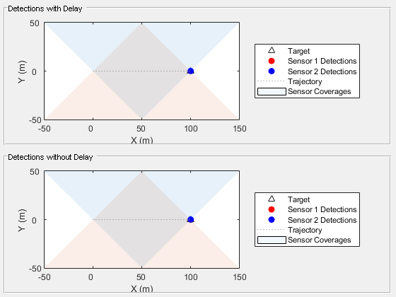
delayer = objectDetectionDelay(SensorIndices = 1, DelaySource = "Input");

Run the following code and observe that the detections from sensor 1 (in red) always lag behind the object. You can also compare the detections with time delay (top) and without time delay (bottom).

while advance(scenario)
    simTime = scenario.SimulationTime;

    % Simulate all the detections from the scenario.
    simDets = detect(scenario);

    % Add a time delay of 1 or 2 simulation steps plus random delay.
    timeDelay = randi(2,1) / scenario.UpdateRate + 0.03 * randn;

    % Apply time delay to the detections.
    delayedDets = delayer(simDets, simTime, timeDelay);

    % Update visualization.
    updateVisualization(tp1, scenario, simDets);
    updateVisualization(tp2, scenario, delayedDets);
end

Summary

In this example, you used the objectDetectionDelay object to simulate out-of-sequence measurements (OOSM). You learned how to control which sensors are affected by the time delay, how to define various random distributions to the delay, and how to use the time delay input argument. You can use the objectDetectionDelay object within a scenario simulation or with recorded data to simulate detections delays.

Supporting Functions

createScenario create a tracking scenario that has one platform with a waypoint trajectory and two radar sensors.

function scenario = createScenario
scenario = trackingScenario(UpdateRate = 10);
% Define a target
platform(scenario, Trajectory = waypointTrajectory([0 0 0; 100 0 0], [0;10]));

% Define a radar with SensorIndex = 1 mounted on one platform
radar1 = fusionRadarSensor(1, "No scanning", MountingAngles = [90 0 0], FieldOfView = [90 5], ...
    RangeResolution = 1, UpdateRate = 10, RangeLimits = [0 200], ...
    DetectionCoordinates  = "Scenario", HasINS = true, HasFalseAlarms = false);
r1p = platform(scenario, Sensors = radar1, Position = [50 -50 0]);
r1p.Signatures{1} = rcsSignature(Pattern = -1e5); % To avoid detection by other radar

% Define a radar with SensorIndex = 2 mounted on another platform
radar2 = fusionRadarSensor(2, "No scanning", MountingAngles = [-90 0 0], FieldOfView = [90 5], ...
    RangeResolution = 1, UpdateRate = 10, RangeLimits = [0 200], ...
    DetectionCoordinates  = "Scenario", HasINS = true, HasFalseAlarms = false);
r2p = platform(scenario, Sensors = radar2, Position = [50 50 0]);
r2p.Signatures{1} = rcsSignature(Pattern = -1e5); % To avoid detection by other radar
end

createVisualization create visualization for the tracking scenario

function [tp1, tp2] = createVisualization(scenario)
f = figure;
p1 = uipanel(f, Title = "Detections without Delay", Position = [0.01 0.01 0.98 0.48]);
p2 = uipanel(f, Title = "Detections with Delay", Position = [0.01 0.51 0.98 0.48]);
a1 = axes(p1);
a2 = axes(p2);
legend(a1, Location = "eastoutside", Orientation = "vertical");
legend(a2, Location = "eastoutside", Orientation = "vertical");
tp1 = theaterPlot(Parent = a1, XLimits = [-50 150], YLimits = [-50 50], ZLimits = [-50 50]);
tp2 = theaterPlot(Parent = a2, XLimits = [-50 150], YLimits = [-50 50], ZLimits = [-50 50]);
platformPlotter(tp1, DisplayName = "Target", Tag = "Target");
platformPlotter(tp2, DisplayName = "Target", Tag = "Target");
detectionPlotter(tp1, DisplayName = "Sensor 1 Detections", Tag = "Sensor1", MarkerEdgeColor = "r", MarkerFaceColor = "r");
detectionPlotter(tp1, DisplayName = "Sensor 2 Detections", Tag = "Sensor2", MarkerEdgeColor = "b", MarkerFaceColor = "b");
detectionPlotter(tp2, DisplayName = "Sensor 1 Detections", Tag = "Sensor1", MarkerEdgeColor = "r", MarkerFaceColor = "r");
detectionPlotter(tp2, DisplayName = "Sensor 2 Detections", Tag = "Sensor2", MarkerEdgeColor = "b", MarkerFaceColor = "b");
trp = trajectoryPlotter(tp1, DisplayName = "Trajectory");
traj = scenario.Platforms{1}.Trajectory;
sampledTimes = traj.TimeOfArrival(1):0.1:traj.TimeOfArrival(end);
pposition = lookupPose(traj,sampledTimes);
plotTrajectory(trp,{pposition});
trp = trajectoryPlotter(tp2, DisplayName = "Trajectory");
traj = scenario.Platforms{1}.Trajectory;
sampledTimes = traj.TimeOfArrival(1):0.1:traj.TimeOfArrival(end);
pposition = lookupPose(traj,sampledTimes);
plotTrajectory(trp,{pposition});
cvp = coveragePlotter(tp1, DisplayName = "Sensor Coverages", Alpha = [0.05 0.05]);
plotCoverage(cvp, coverageConfig(scenario));
cvp = coveragePlotter(tp2, DisplayName = "Sensor Coverages", Alpha = [0.05 0.05]);
plotCoverage(cvp, coverageConfig(scenario));
end

updateVisualization updates the visualization

function updateVisualization(tp, scenario, dets)
tarp = findPlotter(tp, Tag = "Target");
detp1 = findPlotter(tp, Tag = "Sensor1");
detp2 = findPlotter(tp, Tag = "Sensor2");
plotPlatform(tarp, scenario.Platforms{1}.Position);
dets = [dets{:}];
if ~isempty(dets)
    d1 = dets([dets.SensorIndex] == 1);
    plotDetection(detp1, detectionPositions(d1));
    d2 = dets([dets.SensorIndex] == 2);
    plotDetection(detp2, detectionPositions(d2));
end
end

detectionPositions extracts positions from the detections

function pos = detectionPositions(detections)
if ~isempty(detections)
    pos = [detections.Measurement]';
else
    pos = zeros(0,3);
end
end