Use Hardware-Efficient Algorithm to Solve Systems of Complex-Valued Linear Equations

Open Script

This example shows how to solve systems of complex-valued linear equations using hardware-efficient MATLAB® code in Simulink® using a systolic array. The model used in this example shows a hardware-efficient method of solving the system of simultaneous equations

$$AX = B$$

where A is an m-by-n complex matrix, X is an n-by-p complex matrix, and B is an m-by-p complex matrix.

Open Model

Open the fi_complex_mldivide_systolic_array_model model.

model = 'fi_complex_mldivide_systolic_array_model';
open_system(model)

The enabled subsystems that send the data contain MATLAB Function blocks that keep track of which input to send next, and send the rows of matrices A and B to block 4x4 Complex CORDIC Matrix Left Divide when the ready signal is high. If you send data when ready is high, you will not invalidate any data already in the pipeline.

The algorithm overwrites matrix A with an upper-triangular matrix R. The algorithm overwrites B with C = Q'B where Q is unitary and QR = A. The algorithm uses back-substitution on the upper-triangular matrix equation

$$RX = C.$$

To examine the algorithm, look Under the mask of block 4x4 Complex CORDIC Matrix Left Divide.

Define Parameters

Define complex matrices A and B in the base workspace. In this example, matrix A must be 4-by-4, and matrix B must be 4-by-p, where p is the number of right-hand sides.

rng('default');
A = complex(randn(4,4),randn(4,4));
B = complex(randn(4,1),randn(4,1));

The method uses the CORDIC algorithm, so you must also specify the number of iterations of the CORDIC kernel in the NumberOfCORDICIterations parameter, or on the block parameters of the 4x4 Complex CORDIC Matrix Left Divide block.

When A and B are double-precision floating-point data types, set the number of CORDIC iterations to the number of bits in the mantissa of a double. If the inputs are fixed point, then the number of CORDIC iterations must be less than the word length. The accuracy of the computation improves one bit for each iteration, up to the word length of the inputs. This model will work with fixed-point, double, and single data types.

NumberOfCORDICIterations = 52;

You must also instantiate variable BackSubstitutePrototype to specify the data-type used in back-substitution, or enter a prototype value on the block parameters of the "4x4 Complex CORDIC Matrix Left Divide" block. In this case, matrices A and B are double, so set BackSubstitutePrototype value to be a double. This variable is used by the cast function to cast the back-substitute variables using the 'like' syntax.

BackSubstitutePrototype = 0;

Simulate Model

Turn off expected warnings and simulate the model.

warning_state = warning('off','Coder:builtins:ConstantFoldingOverFlow');
sim(model)

After simulation, the model returns matrix X, which is the solution to the matrix equation

$$AX = B$$

Verify the results by checking that AX-B is a small value.

err = norm(A*X - B)

err =

   6.5534e-15

QR Algorithm

The CORDIC algorithm is used to compute the QR decomposition as in the examples Perform QR Factorization Using CORDIC, and Implement Hardware-Efficient QR Decomposition Using CORDIC in a Systolic Array.

This example is of a 4-by-4 matrix A. You can tile the blocks inside this model to build up to any size matrix.

To see the QR algorithm, look under the mask for block Q'B, R 4x4 Complex CORDIC Systolic Array.

Complex QR

Because the data in this example is complex, an additional step is required to zero out the imaginary parts of the pivots to make them real-valued. This is done by splitting the data into real and imaginary parts and using CORDIC to zero out the imaginary part as if it were two rows of a real matrix. This is equivalent to the complex multiplication

$e^{-i\theta} x = r$

where

$
\theta = \tan^{-1}\left({\mbox{\texttt{imag}}(x)\over \mbox{\texttt{real}}(x)}\right)
$

and

$r = \sqrt{\mbox{real}(x)^2 + \mbox{imag}(x)^2}$

except that the computation is done using the CORDIC algorithm without squares or square-roots.

To see the algorithm for $e^{-i\theta} x$ , look under the mask for block Rotate first element to real.

Back-Substitute

Finally, to compute X, compute the reciprocals of the diagonal elements of R and back-substitute into the right-hand side C. The algorithm uses a CORDIC divide implementation to compute the reciprocals.

To see the back-substitute algorithm, look under the mask for block Back Substitute 4x4 Complex CORDIC.

Matrix Inverse

It is usually unnecessary to explicitly compute the inverse of a matrix [3],[5]. However, if you want to do so, set B equal to the identity matrix I. Then, the solution of the equation

$$AX = I$$

equals

$X = A^{-1}.$

A = complex(2*rand(4,4)-1,2*rand(4,4)-1);
B = complex(eye(4));
NumberOfCORDICIterations = 52;
BackSubstitutePrototype = 0;

Simulate the model

sim(model)

Verify that AX and XA are close to the identity matrix. There will be small differences due to round-off errors.

A*X

ans =

   1.0000 + 0.0000i   0.0000 - 0.0000i   0.0000 + 0.0000i   0.0000 - 0.0000i
   0.0000 - 0.0000i   1.0000 + 0.0000i  -0.0000 + 0.0000i  -0.0000 + 0.0000i
  -0.0000 + 0.0000i   0.0000 - 0.0000i   1.0000 + 0.0000i   0.0000 + 0.0000i
   0.0000 + 0.0000i   0.0000 - 0.0000i   0.0000 - 0.0000i   1.0000 - 0.0000i

X*A

ans =

   1.0000 - 0.0000i  -0.0000 - 0.0000i  -0.0000 + 0.0000i   0.0000 - 0.0000i
   0.0000 + 0.0000i   1.0000 + 0.0000i   0.0000 - 0.0000i   0.0000 + 0.0000i
   0.0000 + 0.0000i   0.0000 + 0.0000i   1.0000 - 0.0000i  -0.0000 + 0.0000i
   0.0000 - 0.0000i  -0.0000 + 0.0000i  -0.0000 + 0.0000i   1.0000 + 0.0000i

Fractional Scaling

Normalizing to fractional types makes the computations easier in fixed-point. You can scale the matrices so that their data is in the range [-1, +1] and use fractional fixed-point types because the solution to the matrix equation

$$2^E AX = 2^EB$$

is the same as the solution to

$$AX = B.$$

To convert to fractional scaling with no additional cost in generated code, you can use the reinterpretcast function in MATLAB or the Data Type Conversion block in Simulink with Input and output to have equal Stored Integer.

Run Exhaustive Test Points

You can run many test inputs through the model by making A and B three-dimensional arrays.

m = 4;
n = 4;
p = 1;
n_test_inputs = 100;

Create the inputs such that the real and imaginary parts are in the range [-1, +1]

A = complex(2*rand(m,n,n_test_inputs)-1, 2*rand(m,n,n_test_inputs)-1);
B = complex(2*rand(m,p,n_test_inputs)-1, 2*rand(m,p,n_test_inputs)-1);

In this example, matrices A and B contained real and imaginary parts already in the range [-1, +1], so set the types to be fractional.

data_word_length = 24;
data_fraction_length = 23;

QR Data Types

The growth in the elements of R in the real QR factorization is $\sqrt{m}$ (see Perform QR Factorization Using CORDIC). The elements are complex in this example, so an additional growth factor of $\sqrt{2}$ is needed because

$|1+1i| = \sqrt{2}.$

Also, the CORDIC algorithm grows intermediate values by the following gain factor $K_N$ where $N$ is the number of CORDIC iterations before it is normalized out.

$
K_N = \prod_{j=0}^{N-1}{\sqrt{1+2^{-2j}}} \approx 1.6468
$

Therefore, an upperbound for growth in the QR algorithm for m-by-n complex matrix A is the product of all the growth factors:

$K_N \cdot \sqrt{2m}.$

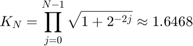
It this example, A is 4-by-4, so the maximum growth factor in the QR algorithm is

$K_n \cdot \sqrt{2m} \approx 1.6468 \cdot \sqrt{2\cdot 4} = 4.6579.$

Therefore, the number of additional integer bits to allow in the QR algorithm to avoid overflow when you have m=4 rows is:

qr_growth_bits = ceil(log2(1.6468*sqrt(2*m)))

qr_growth_bits =

     3

Cast Matrices A and B to Fixed Point

The model requires that the inputs be signed and the word length of B be the same as the word length of A.

Grow the data wordlength to accommodate the QR growth.

qr_input_word_length = data_word_length + qr_growth_bits

qr_input_word_length =

    27

Cast A to fixed point and B to A's type.

T.A = fi([], 1, qr_input_word_length, data_fraction_length);
T.B = T.A;

A = cast(A,'like',T.A);
B = cast(B,'like',T.B);

Back-Substitute Data Type

If $A$ is an $n$ -by- $n$ invertible complex matrix, and $x$ is the solution of matrix equation $Ax=b$ , then using properties of vector and matrix norms (see, for example, reference [6]), it can be shown that

$
||x||_\infty \leq \frac{\sqrt{n}||b||_\infty}{\sigma_n}
$

where $||x||_\infty \equiv \mbox{\texttt{max(abs(x))}}$ and $\sigma_n$ is the smallest singular value of $A$ . This bound is related to the condition number of $A$ .

In this example, $b$ is a complex vector with the real and imaginary parts bounded by 1. Therefore, $||b||_\infty \equiv \mbox{\texttt{max(abs(b))}}\leq \sqrt{2}$ .

Therefore, if you know the distribution of singular values for the $A$ matrices in your problem, then you can choose the number of additional integer bits required to avoid overflow in the back-substitute with a given probability (see, for example, reference [1]).

In this example, we compute the singular values for all the matrices in our test bench and choose the number of integer bits to avoid overflow based on that.

singular_values = zeros(n,n_test_inputs);
A0 = double(A);
for k = 1:n_test_inputs
    singular_values(:,k) = svd(A0(:,:,k));
end
condition_numbers = singular_values(1,:)./singular_values(end,:);
x_bound = sqrt(2*n)./singular_values(end,:);

The number of bits of growth to add is the base-2 logarithm of the maximum bound.

integer_bits_for_backsubstitute = ceil(log2(max(x_bound)))

integer_bits_for_backsubstitute =

     7

Subtract the required integer bits for back-substitute from the wordlength, and an additional bit for the sign bit.

backsubstitute_fraction_length = T.A.WordLength - integer_bits_for_backsubstitute - 1

backsubstitute_fraction_length =

    19

Therefore, the data type for the back-substitute is:

BackSubstitutePrototype = fi(0, 1, T.A.WordLength, backsubstitute_fraction_length)

BackSubstitutePrototype = 

     0

          DataTypeMode: Fixed-point: binary point scaling
            Signedness: Signed
            WordLength: 27
        FractionLength: 19

Set the number of CORDIC iterations to be one less than the fixed-point word length of A.

NumberOfCORDICIterations = T.A.WordLength - 1

NumberOfCORDICIterations =

    26

Simulate the model with fixed-point inputs.

sim(model)

Calculate and Plot the Errors

A measure of error is

norm(AX - B)

for each pair of inputs A and B.

norm_error = zeros(1,size(X,3));
B0 = double(B);
X0 = double(X);
for k = 1:size(X,3)
    norm_error(k) = norm(A0(:,:,k)*X0(:,:,k) - B0(:,:,k));
end

Plot the errors. The errors are low because of the data types chosen. The errors are typically higher when the condition number of matrix A is high, as the theory predicts.

figure(1)
clf
h1 = subplot(2,1,1);
plot(norm_error)
grid on
title('Errors')
ylabel('norm(AX - B)')
h2 = subplot(2,1,2);
plot(condition_numbers)
grid on
title('Condition numbers')
ylabel('cond(A)')
xlabel('Test points')
linkaxes([h1,h2],'x')

Re-enable warnings

warning(warning_state);

References

[1] Zizhong Chen and Jack J. Dongarra. "Condition Numbers of Gaussian Random Matrices". SIAM Journal on Matrix Analysis and Applications. 27.3 (July 2005), pp. 603-620.

[2] George E. Forsythe and Cleve B. Moler. Computer Solution of Linear Algebraic Systems. Englewood Cliffs, N.J.: Prentice-Hall, 1967.

[3] George E. Forsythe, M.A. Malcom and Cleve B. Moler. Computer Methods for Mathematical Computations. Englewood Cliffs, N.J.: Prentice-Hall, 1977.

[4] Cleve B. Moler. Cleve's Corner: What is the Condition Number of a Matrix?>, The MathWorks, Inc. 2017.

[5] Cleve B. Moler. Numerical Computing with MATLAB. SIAM, 2004. isbn: 978-0-898716-60-3.

[6] Gene H. Golub and Charles F. Van Loan. Matrix Computations. The Johns Hopkins University Press.

%#ok<*NOPTS,*NASGU>