Implement HDL-Optimized CORDIC-Based Square Root for Positive Real Numbers

This example shows two implementations of HDL-optimized CORDIC square root in the CORDIC Square Root Resource-Shared block and the CORDIC Square Root Fully-Pipelined block. The first implementation has a resource-shared architecture that is optimized for low hardware utilization. The second implementation has a fully-pipelined architecture that is optimized for high throughput. The core algorithm of both blocks uses CORDIC in hyperbolic vectoring mode to compute the approximation of square root (see Compute Square Root Using CORDIC). This CORDIC-based algorithm is different from the Simulink® Sqrt block, which uses bisection and Newton-Raphson methods. The algorithm in the HDL-optimized CORDIC square root blocks require only iterative shift-add operations.

The input data for this example is a real non-negative scalar. Both blocks use the AMBA AXI handshake protocol at the input and output interfaces.

Generate HDL Code from Resource-Shared Architecture and Fully-Pipelined Architecture

The CORDIC Square Root Resource-Shared block and the CORDIC Square Root Fully-Pipelined block use different architectures for HDL code generation.

Resources-Shared Architecture

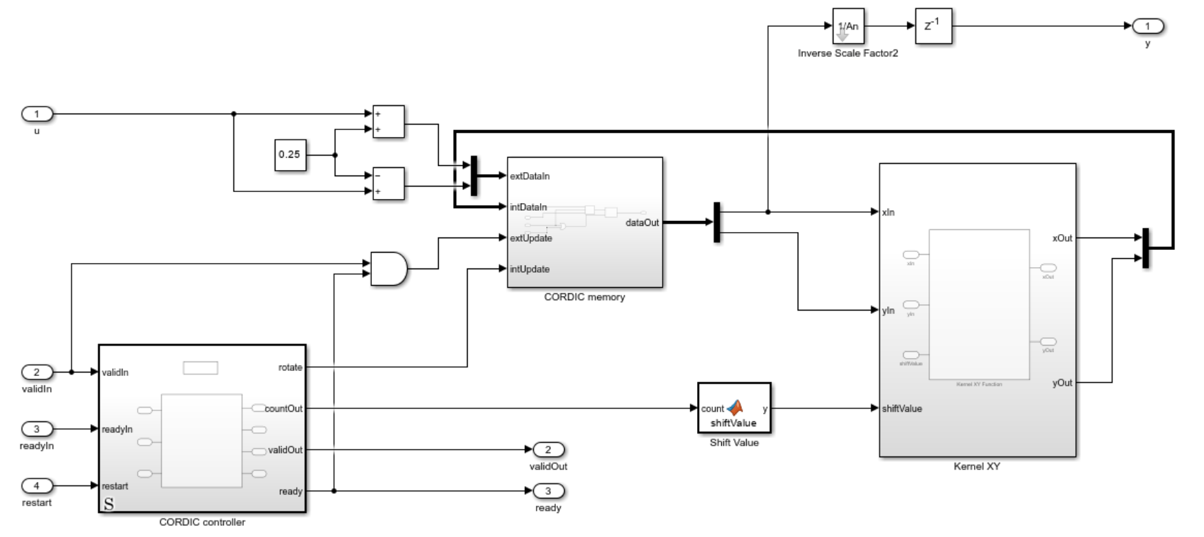
The CORDIC Square Root Resource-Shared block uses a resource-shared architecture. In the generated hardware design, this architecture prioritizes the hardware utilization constraint over throughput. The block has one CORDIC kernel, which is reused for all CORDIC shift-and-add iterations. A controller based on a MATLAB Function block controls the AMBA AXI handshake process and CORDIC workflow. This controller is a Moore machine. The state register and internal counter of the controller are modeled by persistent variables. For guidelines, see Initialize Persistent Variables in MATLAB Functions. The control logic and algorithm data path are intentionally separated for better maintainability and reusability.

Assuming that the upstream block and downstream block are always ready, the block timing diagram is as shown.

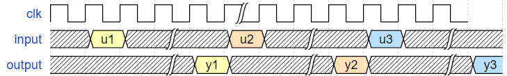
The first u input is u1, u2 is the second u input, y1 is the square root of u1, y2 is the square root of u2, and so on.

After a successful input data transaction, this block starts computing the square root approximation. During the computation, the block ignores all other input data. Once the computation is done, the block holds the result at output port and asserts its validOut signal. After a successful output data transaction, the block becomes ready again. The block asserts its ready signal and waits for the input handshake signal.

Fully-Pipelined Architecture

The CORDIC Square Root Fully-Pipelined block uses a fully-pipelined architecture. In the generated hardware design, this architecture prioritizes throughput over hardware utilization constraints. Each CORDIC shift-and-add iteration is performed by a dedicated CORDIC kernel, so the block can accept new data on any clock cycle if its downstream block is available. The cascaded CORDIC structure is implemented by a for-each subsystem with a Unit Delay Enabled Synchronous block, Selector block, and Mux block. The pipeline registers in the data path are modeled by Unit Delay Enabled Synchronous block so the downstream ready signal can control the data flow. A Unit Delay Enabled Resettable Synchronous block models the pipeline registers in the data path. The downstream ready signal controls the valid signal flow, and the restart signal resets the pipeline registers along the valid signal path.

Assuming that the upstream block and downstream block are always ready, the block timing diagram is as shown.

The first u input is u1, u2 is the second u input, y1 is the square root of u1, y2 is the square root of u2, and so on.

After a successful input data transaction, this block computes the square root approximation of the input data. Because of its fully-pipelined nature, the block is able to accept input data on any cycle, including on consecutive cycles. Once the computation is done, the block holds the result at output port, asserts its validOut signal, and waits for the downstream handshake signal. The ready signal is a direct feedthrough of the readyIn signal for back-pressure propagation. If the downstream block is not ready, this block also pauses accordingly.

Define Simulation Parameters

Specify the number of input samples and data type.

numSamples = 3;

Specify the data type as Fixed, Single, or Double.

DT = 'Fixed';

For fixed-point data type, specify the word length and fraction length.

wordLength = 16;
FractionLength = 10;

Define the maximum CORDIC shift value. In fixed point, this value cannot exceed wordLength - 1.

switch lower(DT)
    case 'fixed'
        maximumShiftValue = wordLength - 1;
    case 'single'
        maximumShiftValue = 23;
    case 'double'
        maximumShiftValue = 52;
    otherwise
        maximumShiftValue = 52;
end

Generate Nonnegative Input u

rng('default');
u = abs(randn(1,numSamples));

Cast to Selected Data Type

switch lower(DT)
    case 'fixed'
        u = cast(u,'like',fi([],1,wordLength,FractionLength));
    case 'single'
        u = single(u);
    case 'double'
        u = double(u);
    otherwise
        u = double(u);
end

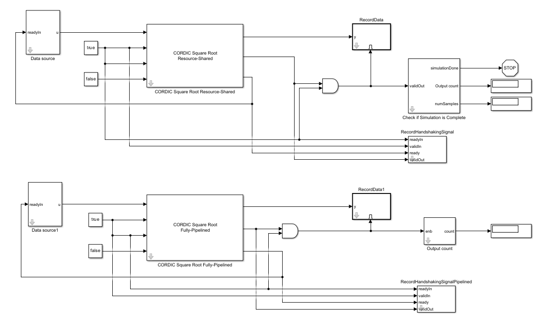
Configure Model Workspace and Run Simulation

model = 'CORDICSquareRootHDLOptimizedModel';
open_system(model);
fixed.example.setModelWorkspace(model,'u',u,'numSamples',numSamples,'maximumShiftValue',maximumShiftValue);
out = sim(model);

Verify Output Solutions

Compare fixed-point results with built-in floating point results.

yBuiltIn = sqrt(double(u))'

yBuiltIn = 3×1

    0.7335
    1.3542
    1.5029

yShared = out.yShared

yShared = 
    0.7334
    1.3535
    1.5029

          DataTypeMode: Fixed-point: binary point scaling
            Signedness: Signed
            WordLength: 16
        FractionLength: 10

yPipelined = out.yPipelined(1:numSamples)

yPipelined = 
    0.7334
    1.3535
    1.5029

          DataTypeMode: Fixed-point: binary point scaling
            Signedness: Signed
            WordLength: 16
        FractionLength: 10

Verify that the CORDIC Square Root Resource-Shared block and the CORDIC Square Root Fully-Pipelined block return identical results in fixed point.

if strcmpi(DT,'fixed')
    yShared == yPipelined %#ok
end

ans = 3x1 logical array

   1
   1
   1

Block Latency Equations

The block latency is the number of clock cycles between a successful input and when the corresponding output becomes valid.

The CORDIC-based square root approximation has two main steps: normalization and CORDIC shift-add iterations. Thus, the total latency is normalization latency plus the latency of the CORDIC shift-add iterations.

The latency of normalization is determined by the input word length.

if isfi(u) && isfixed(u)
    % If input is fi, normalization latency is nextpow2(u.WordLength)+1.
    normLatency = nextpow2(u.WordLength)+1;
else
    % If input is floating point, normalization latency is 0.
    normLatency = 0;
end

The number of CORDIC iterations is determined by the CORDIC maximum shift value. This example uses wordLength - 1 for best precision.

sequence = fixed.cordic.hyperbolic.shiftSequence(maximumShiftValue);
numOfCORDICIterations = length(sequence);

CORDIC Square Root Resource-Shared Block

For the resource-shared architecture, the CORDIC shift-add iterations latency is the number of CORDIC iterations plus two.

blockLatencySharedSim = normLatency + numOfCORDICIterations + 2 %#ok

blockLatencySharedSim = 24

After a successful output, the resource-shared block becomes ready in the next clock cycle.

CORDIC Square Root Fully-Pipelined Block

For the fully-pipelined architecture, the CORDIC shift-add iterations latency is the number of CORDIC iterations plus one.

blockLatencyPipelined = normLatency + numOfCORDICIterations + 1

blockLatencyPipelined = 23

When the downstream block is available, the CORDIC Square Root Fully-Pipelined block can accept new data on any clock cycle, so it is always ready.

Benchmark Block Latency from Simulation

To verify the block latency equations, log the ready/valid handshake signals to measure the block latency in simulation.

validInHistoryShared = out.validInShared;
readyHistoryShared = out.readyShared;
validOutHistoryShared = out.validOutShared;
readyInHistoryShared = out.readyInShared;

validInHistoryPipelined = out.validInPipelined;
readyHistoryPipelined = out.readyPipelined;
validOutHistoryPipelined = out.validOutPipelined;
readyInHistoryPipelined = out.readyInPipelined;

CORDIC Square Root Resource-Shared Block Latency

Find the data transaction time for the CORDIC Square Root Resource-Shared block.

tDataInShared = find(validInHistoryShared & readyHistoryShared == 1);
tDataOutShared = find(validOutHistoryShared & readyInHistoryShared == 1);

Find the rising edge of the ready signal.

tReadyShared = find(diff(readyHistoryShared) == 1) + 1;

Compute the block latency from a successful input to the output.

blockLatencySharedSim = tDataOutShared - tDataInShared(1:numSamples)

blockLatencySharedSim = 3×1

    24
    24
    24

Compute the block latency from a successful output to when the block becomes ready again.

readyLatencySharedSim = tReadyShared - tDataOutShared

readyLatencySharedSim = 3×1

     1
     1
     1

CORDIC Square Root Fully-Pipelined Block Latency

Find the data transaction time.

tDataInPipelined = find(validInHistoryPipelined & readyHistoryPipelined == 1);
tDataOutPipelined = find(validOutHistoryPipelined & readyInHistoryPipelined == 1);

Compute the block latency from a successful into to the corresponding output.

blockLatencyPipelinedSim = tDataOutPipelined(1:numSamples) - tDataInPipelined(1:numSamples)

blockLatencyPipelinedSim = 3×1

    23
    23
    23

Hardware Resource Utilization

Both blocks in this example support HDL code generation using the Simulink® HDL Workflow Advisor. For an example, see HDL Code Generation and FPGA Synthesis from Simulink Model (HDL Coder)(HDL Coder) and Implement Digital Downconverter for FPGA (HDL Coder) (DSP HDL Toolbox).

This example data was generated by synthesizing the block on a Xilinx® Zynq®-7000 SoC ZC702 Evaluation Kit. The synthesis tool was Vivado® v2022.1 (win64).

These parameters were used for synthesis:

• Input data type: sfix16_En10

• maximumShiftValue: 15 (WordLength - 1)

• Target frequency: 200 MHz

This table shows the post-place-and-route resource utilization results for the CORDIC Square Root Resource-Shared block.

Resource	Usage	Available	Utilization (%)
Slice LUTs	445	53200	0.84
Slice Registers	92	106400	0.09
DSPs	0	220	0.00
Block RAM Tile	0	140	0.00

This table shows the timing summary for the CORDIC Square Root Resource-Shared block.

	Value
Requirement	5 ns (200 MHz)
Data Path Delay	5.337 ns
Slack	-0.312 ns
Clock Frequency	184.71 MHz

This table shows the post-place-and-route resource utilization results for the CORDIC Square Root Fully-Pipelined block.

Resource	Usage	Available	Utilization (%)
Slice LUTs	926	53200	1.74
Slice Registers	701	106400	0.66
DSPs	0	220	0.00
Block RAM Tile	0	140	0.00

This table shows the timing summary for the CORDIC Square Root Fully-Pipelined block.

	Value
Requirement	5 ns (200 MHz)
Data Path Delay	5.016 ns
Slack	0.009 ns
Clock Frequency	200.36 MHz

Related Topics

• Compute Square Root Using CORDIC