Compute SVD of Non-Square Matrices Using Square Jacobi SVD HDL Optimized Block by Forming Covariance Matrices

This example shows how to use the Square Jacobi SVD HDL Optimized block to compute the singular value decomposition (SVD) of non-square matrices by forming covariance matrices.

Compute SVD of Non-Square Matrices by Forming Covariance Matrices

The Square Jacobi SVD HDL Optimized block can perform singular value decomposition of square matrices. If the input is non-square matrices, there are two preprocesses that can transform the non-square matrices into square matrices. The first one is QR decomposition and the Non-Square Jacobi SVD HDL Optimized utilizes this method. This example shows the second method that forms the square covariance matrices before computing the SVD. Comparing to the QR decomposition, this method can have smaller latency in the generated hardware. The costs are more multipliers and the word length in the following square SVD computation is twice of that with QR decomposition.

HDL code generation

Square Jacobi HDL Optimized block supports bit and cycle true HDL code generation. To generate HDL code of this example, you can use HDL Block Properties: General (HDL Coder) to configure the code generation behavior of the matrix multiply block. To use this example as it is, set the DotProductStractegy to Fully Parallel Scalarized such that the multiplication introduce zero latency.

Define Simulation Parameters

Specify the dimension of the sample matrices, the number of input sample matrices, and the number of iterations of the Jacobi algorithm.

m = 16;
n = 8;
numSamples = 3;
nIterations = 10;

Generate Input A Matrices

Use the specified simulation parameters to generate the input matrix A.

rng('default');
A = randn(m,n,numSamples);

The Non-Square Jacobi SVD HDL Optimized block supports both real and complex inputs. Set the complexity of the input in the block mask accordingly.

% A = complex(randn(m,n,numSamples),randn(m,n,numSamples));

Select Fixed-Point Data Types

Define the desired word length.

wordLength = 32;

Use the upper bound on the singular values to define fixed-point types that will never overflow. First, use the fixed.singularValueUpperBound function to determine the upper bound on the singular values.

svdUpperBound = fixed.singularValueUpperBound(m,n,max(abs(A(:))));

Define the integer length based on the value of the upper bound, with one additional bit for the sign, another additional bit for intermediate CORDIC growth, and one more bit for intermediate growth to compute the Jacobi rotations.

additionalBitGrowth = 3;
integerLength = ceil(log2(svdUpperBound)) + additionalBitGrowth;

Compute the fraction length based on the integer length and the desired word length.

fractionLength = wordLength - integerLength;

Define the signed fixed-point data type to be 'Fixed' or 'ScaledDouble'. You can also define the type to be 'double' or 'single'.

dataType = 'Fixed';
T.A = fi([],1,wordLength,fractionLength,'DataType',dataType);
disp(T.A)

[]

          DataTypeMode: Fixed-point: binary point scaling
            Signedness: Signed
            WordLength: 32
        FractionLength: 23

Cast the matrix A to the signed fixed-point type.

A = cast(A,'like',T.A);

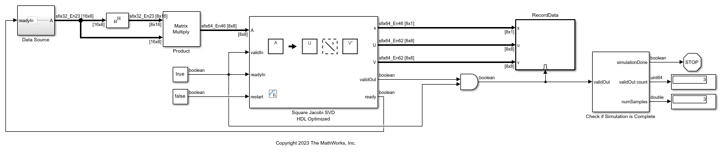
Configure Model Workspace and Run Simulation

model = 'SquareJacobiSVDWithCovarianceMatModel';
open_system(model);
fixed.example.setModelWorkspace(model,'A',A,'m',m,'n',n,...
    'nIterations',nIterations,'numSamples',numSamples);
out = sim(model);

Verify Output Solutions

Verify the output solutions. In these steps, "identical" means within roundoff error.

The word length is twice of the input matrices' to maintain same precision after forming the covariance matrices.

disp(numerictype(out.s));

          DataTypeMode: Fixed-point: binary point scaling
            Signedness: Signed
            WordLength: 64
        FractionLength: 46

1. Verify that U*diag(s)*V' is identical to A'*A. relativeErrorUSV represents the relative error between U*diag(s)*V' and A'*A.

2. Verify that the square root of singular values s are identical to the floating-point SVD solution. relativeErrorS represents the relative error between sqrt(s) and the singular values calculated by the MATLAB® svd function.

3. Verify that U and V are unitary matrices. relativeErrorUU represents the relative error between U'*U and the identity matrix. relativeErrorVV represents the relative error between V'*V and the identity matrix.

for i = 1:numSamples
    disp(['Sample #',num2str(i),':']);
    a = A(:,:,i);
    U = out.U(:,:,i);
    V = out.V(:,:,i);
    s = out.s(:,:,i);

    % Verify U*diag(s)*V'
    if norm(double(a)) > 1
        relativeErrorUSV = norm(double(U*diag(s)*V')-double(a'*a))/norm(double(a'*a));
    else
        relativeErrorUSV = norm(double(U*diag(s)*V')-double(a'*a));
    end
    relativeErrorUSV %#ok

    % Verify s
    s_expected = svd(double(a'*a));
    normS = norm(s_expected);
    relativeErrorS = norm(double(s) - s_expected);
    if normS > 1
        relativeErrorS = relativeErrorS/normS;
    end
    relativeErrorS %#ok

    % Verify U'*U
    U = double(U);
    UU = U'*U;
    relativeErrorUU = norm(UU - eye(size(UU))) %#ok

    % Verify V'*V
    V = double(V);
    VV = V'*V;
    relativeErrorVV = norm(VV - eye(size(VV))) %#ok

    disp('---------------');

end

Sample #1:

relativeErrorUSV =

   1.6151e-13


relativeErrorS =

   3.8078e-14


relativeErrorUU =

   1.8078e-14


relativeErrorVV =

   1.8060e-14

---------------
Sample #2:

relativeErrorUSV =

   2.9196e-13


relativeErrorS =

   6.3936e-14


relativeErrorUU =

   1.8252e-14


relativeErrorVV =

   1.8097e-14

---------------
Sample #3:

relativeErrorUSV =

   2.2967e-13


relativeErrorS =

   4.9331e-14


relativeErrorUU =

   1.8223e-14


relativeErrorVV =

   1.8044e-14

---------------