Simulate Conditional Mean and Variance Models

This example shows how to simulate responses and conditional variances from a composite conditional mean and variance model.

Load the Data and Fit a Model

Load the NASDAQ data included with the toolbox. Fit a conditional mean and variance model to the daily returns. Scale the returns to percentage returns for numerical stability

load Data_EquityIdx
nasdaq = DataTable.NASDAQ;
r = 100*price2ret(nasdaq);
T = length(r);

Mdl = arima('ARLags',1,'Variance',garch(1,1),...
    'Distribution','t');
EstMdl = estimate(Mdl,r,'Variance0',{'Constant0',0.001});

 
    ARIMA(1,0,0) Model (t Distribution):
 
                 Value      StandardError    TStatistic      PValue  
                ________    _____________    __________    __________

    Constant    0.093488      0.016694         5.6002      2.1414e-08
    AR{1}        0.13911      0.018857         7.3771      1.6175e-13
    DoF           7.4775       0.88261          8.472      2.4126e-17

 
 
    GARCH(1,1) Conditional Variance Model (t Distribution):
 
                 Value      StandardError    TStatistic      PValue  
                ________    _____________    __________    __________

    Constant    0.011246      0.0036305        3.0976       0.0019511
    GARCH{1}     0.90766       0.010516        86.315               0
    ARCH{1}     0.089897       0.010835        8.2966      1.0712e-16
    DoF           7.4775        0.88261         8.472      2.4126e-17

[e0,v0] = infer(EstMdl,r);

Simulate Returns, Innovations, and Conditional Variances

Use simulate to generate 100 sample paths for the returns, innovations, and conditional variances for a 1000-period future horizon. Use the observed returns and inferred residuals and conditional variances as presample data.

rng 'default';
[y,e,v] = simulate(EstMdl,1000,'NumPaths',100,...
    'Y0',r,'E0',e0,'V0',v0);

figure
plot(r)
hold on
plot(T+1:T+1000,y)
xlim([0,T+1000])
title('Simulated Returns')
hold off

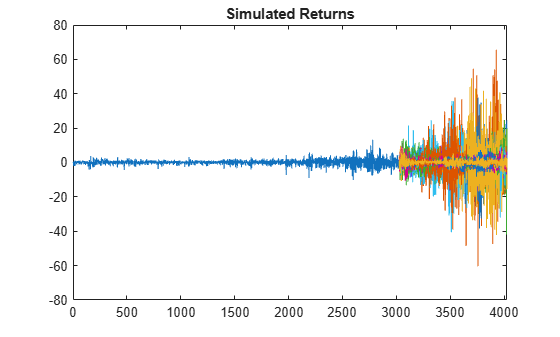
The simulation shows increased volatility over the forecast horizon.

Plot Conditional Variances

Plot the inferred and simulated conditional variances.

figure
plot(v0)
hold on
plot(T+1:T+1000,v)
xlim([0,T+1000])
title('Simulated Conditional Variances')
hold off

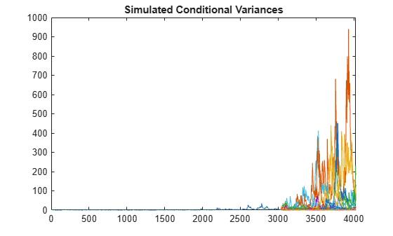
The increased volatility in the simulated returns is due to larger conditional variances over the forecast horizon.

Plot Standardized Innovations

Standardize the innovations using the square root of the conditional variance process. Plot the standardized innovations over the forecast horizon.

figure
plot(e./sqrt(v))
xlim([0,1000])
title('Simulated Standardized Innovations')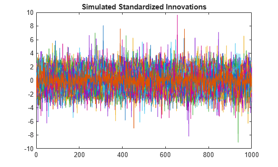

The fitted model assumes the standardized innovations follow a standardized Student's t distribution. Thus, the simulated innovations have more larger values than would be expected from a Gaussian innovation distribution.