Model Seasonal Lag Effects Using Indicator Variables
This example shows how to estimate a seasonal ARIMA model:
Model the seasonal effects using a multiplicative seasonal model.
Use indicator variables as a regression component for the seasonal effects, called seasonal dummies.
Subsequently, their forecasts show that the methods produce similar results. The time series is monthly international airline passenger numbers from 1949 to 1960.
Load Data
Load the data set Data_Airline, and plot the natural log of the monthly passenger totals counts.
load Data_Airline
dat = log(DataTimeTable.PSSG); % Transform to logarithmic scale
T = size(dat,1);
y = dat(1:103);  % Estimation sample
y is the part of dat used for estimation, and the rest of dat is the holdout sample to compare the two models' forecasts.
Fit Seasonal-Lag Model
Create an ARIMA model
where is an independent and identically distributed normally distributed series with mean 0 and variance . Use estimate to fit Mdl1 to y.
Mdl1 = arima('Constant',0,'MALags',1,'D',1,...
    'SMALags',12,'Seasonality',12);
EstMdl1 = estimate(Mdl1,y);
    ARIMA(0,1,1) Model Seasonally Integrated with Seasonal MA(12) (Gaussian Distribution):

                 Value      StandardError    TStatistic      PValue
                ________    _____________    __________    __________

    Constant           0              0           NaN             NaN
    MA{1}       -0.35732       0.088031        -4.059      4.9286e-05
    SMA{12}     -0.61469       0.096249       -6.3864      1.6985e-10
    Variance    0.001305      0.0001527        8.5467      1.2671e-17
The fitted model is
where is an iid normally distributed series with mean 0 and variance 0.0013.
Fit Seasonal-Dummy Model
Create an ARIMAX(0,1,1) model with period 12 seasonal differencing and a regression component,
is a series of T column vectors having length 12 that indicate in which month observation was measured. A 1 in row i of indicates that the observation was measured in month i, the rest of the elements are 0s.
Note that if you include an additive constant in the model, then the T rows of the design matrix X are composed of the row vectors . Therefore, X is rank deficient, and one regression coefficient is not identifiable. A constant is left out of this example to avoid distraction from the main purpose. Format the in-sample X matrix
X  = dummyvar(repmat((1:12)',12,1));

% Format the presample X matrix
X0 = [zeros(1,11) 1; dummyvar((1:12)')];
Mdl2 = arima('Constant',0,'MALags',1,'D',1,...
    'Seasonality',12);
EstMdl2   = estimate(Mdl2,y,'X',[X0; X]);
    ARIMAX(0,1,1) Model Seasonally Integrated (Gaussian Distribution):

                  Value       StandardError    TStatistic      PValue
                __________    _____________    __________    __________

    Constant             0              0            NaN            NaN
    MA{1}         -0.40711       0.084387        -4.8242     1.4053e-06
    Beta(1)      -0.002577       0.025168       -0.10239        0.91845
    Beta(2)     -0.0057769       0.031885       -0.18118        0.85623
    Beta(3)     -0.0022034       0.030527      -0.072179        0.94246
    Beta(4)     0.00094737       0.019867       0.047687        0.96197
    Beta(5)     -0.0012146       0.017981      -0.067551        0.94614
    Beta(6)        0.00487       0.018374        0.26505        0.79097
    Beta(7)     -0.0087944       0.015285       -0.57535        0.56505
    Beta(8)      0.0048346       0.012484        0.38728        0.69855
    Beta(9)       0.001437       0.018245       0.078758        0.93722
    Beta(10)      0.009274       0.014751        0.62869        0.52955
    Beta(11)     0.0073665         0.0105        0.70158        0.48294
    Beta(12)    0.00098841       0.014295       0.069146        0.94487
    Variance     0.0017715     0.00024657         7.1848     6.7329e-13
The fitted model is
where is an iid normally distributed series with mean 0 and variance 0.0017 and is a column vector with the values Beta1 - Beta12. Note that the estimates MA{1} and Variance between Mdl1 and Mdl2 are not equal.
Forecast Both Models
Use forecast to forecast both models 41 periods into the future from July 1957. Plot the holdout sample using these forecasts.
fT = 41;
fh = DataTimeTable.Time((end-fT+1):end);

yF1 = forecast(EstMdl1,41,y);
yF2 = forecast(EstMdl2,41,y,'X0',X(1:103,:),'XF',X(104:end,:));
l1 = plot(DataTimeTable.Time(100:end),dat(100:end),'k','LineWidth',3);
hold on
l2 = plot(fh,yF1,'-r','LineWidth',2);
l3 = plot(fh,yF2,'-b','LineWidth',2);
hold off
title('Passenger Data: Actual vs. Forecasts')
xlabel('Month')
ylabel('Logarithm of Monthly Passenger Data')
legend({'Observations','Polynomial Forecast',...
 			'Regression Forecast'},'Location','NorthWest')
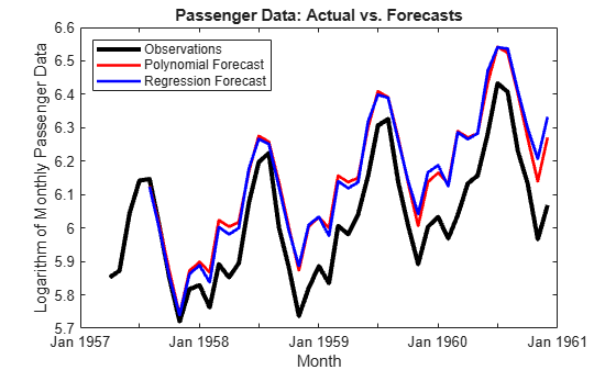
Though they overpredict the holdout observations, the forecasts of both models are almost equivalent. One main difference between the models is that EstMdl1 is more parsimonious than EstMdl2.
References:
Box, G. E. P., G. M. Jenkins, and G. C. Reinsel. Time Series Analysis: Forecasting and Control. 3rd ed. Englewood Cliffs, NJ: Prentice Hall, 1994.
See Also
Objects
Functions
Topics
- Create Seasonal ARIMA (SARIMA) Model for Time Series Data
- Estimate Seasonal ARIMA (SARIMA) Model
- Forecast Multiplicative ARIMA Model
- Check Fit of Multiplicative ARIMA Model
- Forecast IGD Rate from ARX Model
- Create Seasonal ARIMA (SARIMA) Models
- Create ARIMA Models That Include Exogenous Covariates
- Conditional Mean Model Estimation with Equality Constraints
- Forecast Conditional Mean Model Programmatically