Assess State-Space Model Stability Using Rolling Window Analysis
Assess Model Stability Using Rolling Window Analysis
This example shows how to use a rolling window to check whether the parameters of a time-series model are time invariant. This example analyzes two time series:
Time-series 1: simulated data from a known, time-invariant model
Time-series 2: simulated data from a known, time-varying model
Completely specify this AR(1) model for Time-series 1:
where is Gaussian with mean 0 and variance 1. Completely specify this time-varying model for Time-series 2:
where is Gaussian with mean 0 and variance 1.
Mdl1 = arima('AR',0.6,'Constant',0,'Variance',1);

Mdl2 = cell(3,1); % Preallocate
ARMdl2 = [0.2 0.75 -0.5];
for j = 1:3
    Mdl2{j} = arima('AR',ARMdl2(j),'Constant',0,'Variance',1);
end
Mdl1 is an arima model objects. You can access its properties using dot notation. Mdl2 is a cell array of arima model objects. You can you cell indexing and dot notation to access properties of the models within Mdl2. For example, to access the AR parameter value of the third model in Mdl3, enter Mdl2{3}.AR.
Simulate T = 200 periods of data from Mdl1 and Mdl2. Use a presample response of 0 for both series.
rng(1); % For reproducibility
T = 200;
y1 = simulate(Mdl1,T,'Y0',0);
timeMdl2 = [100 50 50]; % Number of observations per model in Mdl2
y2 = 0;
for k = 1:numel(Mdl2)
    y2 = [y2; simulate(Mdl2{k},timeMdl2(k),'Y0',y2(end))];
end

Y = [y1 y2(2:end)];
Specify empty AR(1) models for the estimation of Mdl1, Mdl2, and Mdl3. Estimate all three models using the respective data sets and a rolling window size of 40 periods. Also, use a rolling window increment of one period. Store the autoregressive parameters and estimated innovations variance.
Mdl = arima('ARLags',1,'Constant',0);

m = 100;       % Rolling window size
N = T - m + 1; % Number of rolling windows

EstParams = cell(2,1);     % Preallocate for estimates
EstParamsMat = zeros(N,2);
EstParamsSE = cell(2,1);
EstParamsSEMat = zeros(N,2);

for j = 1:2
    for k = 1:N
        idxRW =  k:(m + k - 1); % In-sample indices
        [EstMdl,EstParamCov] = estimate(Mdl,Y(idxRW,j),'Display','off');
        EstParamsMat(k,:) = [EstMdl.AR{1} EstMdl.Variance];
        EstParamsSEMat(k,:) = sqrt([EstParamCov(2,2) EstParamCov(3,3)]);
    end
    EstParams{j} = EstParamsMat;
    EstParamsSE{j} = EstParamsSEMat;
end
Plot the estimates and their point-wise confidence intervals over the rolling window index.
titleMdls = {'Mdl1','Mdl2'};

for j = 1:2
    figure;
    subplot(2,1,1);
    Estimates = EstParams{j};
    SEs = EstParamsSE{j};
    plot(Estimates(:,1),'LineWidth',2);
    hold on;
    plot(Estimates(:,1) + 2*SEs(:,1),'r:','LineWidth',2);
    plot(Estimates(:,1) - 2*SEs(:,1),'r:','LineWidth',2);
    title(sprintf('%s - AR at Lag 1 Estimate',titleMdls{j}));
    xlabel 'Rolling window index';
    axis tight;
    hold off;
    subplot(2,1,2);
    plot(Estimates(:,2),'LineWidth',2);
    hold on;
    plot(Estimates (:,2) + 2*SEs(:,2),'r:','LineWidth',2);
    plot(Estimates(:,2) - 2*SEs(:,2),'r:','LineWidth',2);
    title(sprintf('%s - Variance Estimate',titleMdls{j}));
    xlabel 'Rolling window index';
    axis tight;
    hold off;
end

For Mdl1, the AR estimate does not vary much from 0.6, and the estimates are not significantly different from one another (pair-wise). Similar results occur for the variance of Mdl1. The AR estimate of Mdl2 grows, and then falls, which indicates time dependence. Also, based on the confidence intervals, there is evidence that some estimates differ from others. Though the variance did not change during simulation, there seems to be heteroscedasticity possibly induced by the instability of the model.
Assess Stability of Implicitly Created State-Space Model
This example shows how to specify and estimate a state space model when conducting a rolling window analysis for stability. A rolling window analysis for an explicitly defined state-space model is straightforward, so this example focuses on implicitly defined state-space models.
Consider this state-space model:
where εt and
ut are Gaussian process
with mean 0 and variance 1. Create the function
rwParamMap.m, which specifies how the parameters in
params map to the state-space model matrices, the
initial state values, and the type of state, and save it in your working
folder.
function [A,B,C,D,Mean0,Cov0,StateType,deflateY] = rwParamMap(params,y,Z)
%rwParamMap Parameter-to-matrix mapping function for rolling window example
%using ssm
%   The state space model specified by rwParamMap contains a stationary
%   AR(1) state, the observation model includes a regression component, and
%   the variances of the innovation and disturbances are 1. The response y
%   is deflated by the regression component specified by the predictor
%   variables x.
A = params(1);
B = 1;
C = 1;
D = 1;
Mean0 = [];
Cov0 = [];
StateType = 0;
deflateY = y - params(2)*Z;
end
The software does not support the simulation of implicit models containing a regression component. Therefore, to simulate data from this model, you must specify all model components up to the regression component. You can do this explicitly since this example uses a simple state-space model. Otherwise, you can create another function and define another state-space model implicitly (e.g., for time-varying state-space models).
Mdl2Sim = ssm(NaN,1,1,1,'StateType',1);Mdl2Sim is an implicitly defined ssm object.
Simulate a 200-period path of random standard Gaussian data. Then,
simulate responses from Mdl2Sim, and inflate the
responses with the regression component. For this example, use
ϕ = 0.6 and β = 2.
rng(1); % For reproducibility
T = 200;
Z = randn(T,1);
phi = 0.6;
beta = 2;
deflateY = simulate(Mdl2Sim,T,'Params',phi);
y = deflateY + Z*beta;
y is the inflated, simulated response path, and
Z is the simulated predictor series.
If you define a state-space model implicitly and the response and
predictor data (i.e., y and Z) exist
in the MATLAB® Workspace, then the software creates a link from the
parameter-to-matrix mapping function those series. If the data do not exist
in the MATLAB Workspace, then the software creates the model, but you must
provide the data using the appropriate name-value pair arguments when you,
e.g., estimate the model.
Therefore, to conduct a rolling window analysis when the state-space model is implicitly defined and there is a regression component, you must specify the state-space model indicating the indices of the data to be analyzed for each window. Conduct a rolling window analysis of the simulated data. Let the rolling window length be 100 periods for this example.
m = 100;
N = T - m + 1;        % Number of rolling windows

EstParams = nan(N,2); % Preallocation
EstParamSE = nan(N,2);

for j = 1:N;
    idxRW = j:(m + j - 1);
    Mdl = ssm(@(c)rwParamMap(c,y(idxRW),Z(idxRW)));
    [~,EstParams(j,:),EstParamCov] = estimate(Mdl,y(idxRW),[0.5 1]',...
        'Display','off');
    EstParamSE(j,:) = sqrt(diag(EstParamCov));
end
Plot the estimates and point-wise confidence intervals for the AR parameter and regression coefficient.
figure;
subplot(2,1,1);
plot(EstParams(:,1),'LineWidth',2);
hold on;
plot(EstParams(:,1) + 2*EstParamSE(:,1),':r','LineWidth',2);
plot(EstParams(:,1) - 2*EstParamSE(:,1),':r','LineWidth',2);
title 'State AR Estimate at Lag 1';
xlabel 'Rolling window index';
axis tight;
hold off;
subplot(2,1,2);
plot(EstParams(:,2),'LineWidth',2);
hold on;
plot(EstParams(:,2) + 2*EstParamSE(:,2),':r','LineWidth',2);
plot(EstParams(:,2) - 2*EstParamSE(:,2),':r','LineWidth',2);
title 'Regression Coefficient Estimate';
xlabel 'Rolling window index';
axis tight;
hold off;
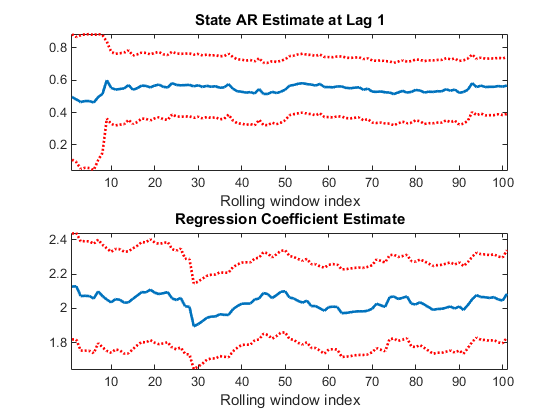
The plots indicate that the model is stable since the AR estimate does not deviate much from its mean, nor does the regression coefficient estimate.