Rectangular Array MVDR Beamformer
This example shows how to implement a minimum-variance distortionless-response (MVDR) beamformer for a 4x4 rectangular antenna array on FPGA.
MVDR (Minimum Variance Distortionless Response) beamforming is a signal processing technique used in radar applications to enhance the detection and tracking of targets while suppressing interference and noise from other sources. The goal of beamforming is to improve the radar's spatial resolution and target detection capabilities. The MVDR beamforming algorithm provides maximum signal to noise in the direction of the desired target and minimum output power in the directions of interference and noise.
Introduction
This example uses MVDR beamforming to improve the detection and tracking of a target in the presence of interference and noise. Assume that the target is being tracked by a radar system consisting of an array of antennas placed in a rectangular array. The received radar signal will be corrupted by noise and interference from other sources. The MVDR beamforming algorithm aligns the antenna array with the direction of the target and suppresses noise and interference from other directions.
The 4x4 antenna geometry has each antenna element spaced by lambda/2 so all the elements of the array are on coordinates of +/-3/4 or +/-1/4 lambda. The antenna is oriented so that the boresight is aligned with x axis and the array is centered around 0,0 in the y,z plane. Using the pattern method of the sensor array, you can plot the normalized antenna response. This antenna does not have a counterpoise (ground plane) or back baffle behind the elements so it is sensitive to signals from both the positive and negative x axis directions, but Phased Array System Toolbox™ only allows for steering angles in the positive x direction. You can change the antenna elements to add back baffling, if needed.
The steering vector angles for this antenna indicate the direction to maximize signal from that direction and minimize interference from other directions. The direction you choose for the steering vector has a very large effect on your ability to receive the return signal and a few degrees of misalignment can make the received signal undecodeable. The antenna can be steered in both azimuth and elevation, but this example steers only the azimuth.
Beamformer Behavioral Model
The MVDR beamformer preserves the gain in the direction of arrival of a desired signal and attenuates interference from other directions [1].

Input Signals, Frequencies, and Directions
This model sets up a single primary signal and a single interfering signal, using a frame size of 800 samples. The Narrowband Rx Array block combines these signals, along with their respective source angles of 20 and 60 degrees azimuth with an implied 0 degree elevation. The block uses the 4x4 sensor array from the initialization file and an operating frequency of 915 MHz. The output of the Narrowband Rx Array block is a vector of signals from the sensor array with the geometry of the source angles applied. This vector is sent to the Receiver Preamp which reduces the signal, simulating return loss, and adds phase noise.
In order to better match the HDL algorithm, the resulting output is quantized to a 12-bit fixed-point value and then converted back to double precision. This conversion allows you to model the quantization effects in the double-precision behavioral model of the MVDR algorithm.
Behavioral Model in MATLAB
The behavioral algorithm in MATLAB® is the classic MVDR algorithm where the covariance matrix is formed by multiplying the input by its conjugate. The covariance matrix is then used with the backslash or mldivide operator and the steering vector to solve the set of equations  where
where  is the covariance matrix,
  is the steering vector, and
  is the weight vector for the MVDR beamformer. The weight vector is then normalized and the normalized vector is conjugated and multiplied by the input to apply the beamforming and steering.

Computing the Response in MATLAB
Given readings from a sensor array, such as the uniform rectangular array (URA) in the following diagram, form data matrix from samples of the array, where  is an
is an  -by-1 column vector of readings from the array sampled at time
  , and
, and  is one row of matrix . Many more samples are taken than there are elements in the array. This sampling results in the number of rows in being much greater than the number of columns. An estimate of the covariance matrix is
  , where
  is the Hermitian or complex-conjugate transpose of .
Compute the MVDR beamformer response by solving the following equation for , where is a steering vector pointing in the direction of the desired signal.

The MVDR weight vector  is computed from and using the following equation, which normalizes to preserve the gain in the direction of arrival of the desired signal.

The MVDR system response is the inner product of the MVDR weight vector and a current sample from the sensor array .

The MVDR beamforming algorithm does not depend on the antenna geometry. The antenna geometry is captured in the supplied steering vector, but the algorithm works only with the variance between channels.

Hardware-Friendly Algorithm
Instead of forming data matrix and computing the Cholesky factorization of covariance matrix , the upper-triangular matrix of the QR decomposition of is computed directly and updated as each data vector streams in from the sensor array. Because the data is updated indefinitely, a forgetting factor is applied after each factorization. To integrate with an equivalent of a matrix of  rows, the forgetting factor
  should be set to

This example simulates the equivalent of a matrix with  rows, so the forgetting factor is set to 0.9983.
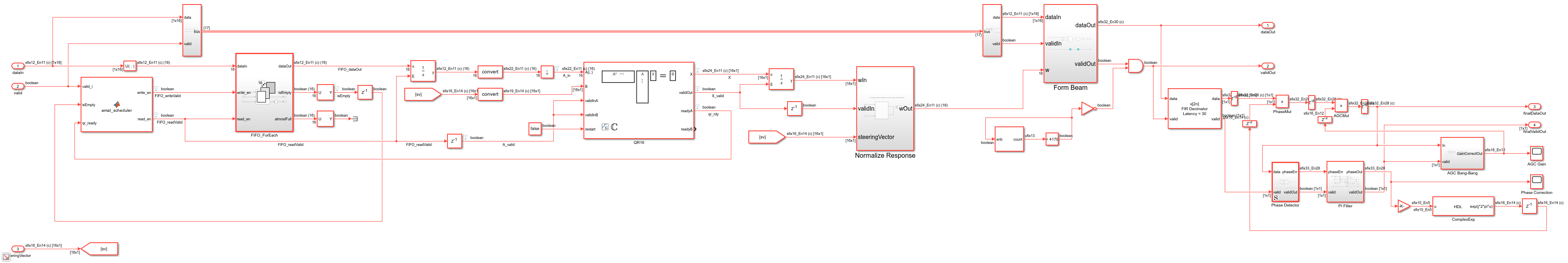
The Complex Partial-Systolic Matrix Solve Using Q-less QR Decomposition with Forgetting Factor block is implemented using the method shown in the example "FPGA-Based Minimum-Variance Distortionless-Response (MVDR) Beamformer". The upper-triangular matrix  from the QR decomposition of is identical to the Cholesky factorization of except the signs of values on the diagonal. Solving the matrix equation
  by computing the Cholesky factorization of is not as efficient or as numerically sound as computing the QR decomposition of directly.
After the beamingforming operations, you are left with a two-times oversampled QPSK signal that you can filter and decode. Implementing the raised cosine receive filter in an FPGA is very straightforward. You get the filter coefficients from the initialization code and you can view them in the behavioral received filter by opening the block and clicking on the "View Filter Response" button. This filter is a 21-tap decimate by two FIR filter with an initial latency of 30 cycles. The valid control signal into the filter is continuously high after the latency of the beamformer, but since the filter decimates the input, the output valid of the filter is high only every other cycle.
From the filter, the data is passed through the phase rotation multiplier and AGC multiplier to a Phase Detector built out of basic blocks. Since the Phased-Array Toolbox operates on baseband signals, there is no carrier to remove with the classic QPSK Costas loop, but using the sign-bit to take either the input signal real and imaginary components or their negations allows the phase detector to output a phase error signal proportional to the required phase rotation to place the QPSK constellation back on the correct axis. This phase error is then passed to proportional-integral (PI) filter and the result is integrated into a phase output.

Phase Correction
The phase output must be corrected by multiplying by  to get the normalized phase needed for the HDL-optimized complex exponential block. The sine and cosine output from the complex exponential block, as a complex number, is then used to phase rotate the original filter output, putting the QPSK back on the correct constellation points. This operation completes the phase correction feedback look.

Gain Correction
The signal is also passed through automatic gain control (AGC). The AGC is a "bang-bang" controller with just hysteresis between the upper and lower thresholds. In practice the AGC for a QPSK signal just needs to spread the constellation enough to enable correct sign-bit-based data thresholding. The input to the AGC is separated into real and imaginary parts and each part is squared and then summed to form an estimate of the signal power. You need to low-pass filter the result and decimate it so that the AGC adjusts the gain with a slower period. You accomplish this filter and decimation with a CIC decimating filter that decimates the power input by 100. You then compare the decimated result to the upper and lower limits.
In a normalized QPSK signal, the center of each constellation point is  from the center in both X and Y dimensions, which means the vector distance to the center is 1.0. In the power domain of the CIC filter output, the upper and lower limits are slightly above and below sqrt(2), since the filter output is already the sum of the squares of the input real and imaginary parts. The example shows a +/-2.5% hysteresis band for these limits to compare with the filter output. You then use an up/down counter with an enable using the MATLAB Function block. The counter will change anytime the power is outside the given range and the direction it changes depends on whether the upper or lower limit is exceeded. You use the counter output to index a table of gain values. You choose 0.5 dB steps starting from 0.5 dB of gain up to 16 dB of gain, for a total of 32 steps. The AGC multiplier uses the output of this gain table, completing the AGC loop.

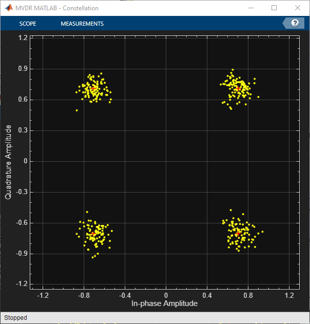
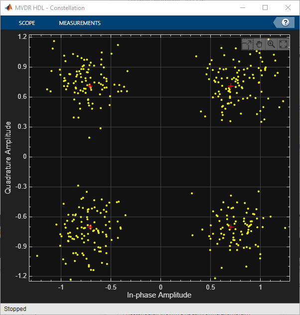
Results
Simulating this model, you can see the QPSK constellations similar to the figures shown here. The performance of the hardware-friendly subsystem is not quite as good as the double-precision behavioral model, but is acceptable. Some of the differences between the two can be attributed to the fixed-point quantization, the differences in the QPSK decoder, and the differences in the AGC in the hardware-friendly subsystem.
Going Further
The Phased Array System Toolbox does a simplified baseband or IF simulation of radar systems, so adding more RF processing to the model would help to make the HDL portion of the design closer to the final form.
You could do the steering vector computation in HDL as well. This operation requires sine and cosine computations on the azimuth and elevation and some simple geometry for the array coordinates.
The QPSK data for the radar signal can be used to carry information and you could decode and display that information.
References
[1] C.M. Rader. "VLSI Systolic Arrays for Adaptive Nulling". In: IEEE Signal Processing Magazine (July 1996), pp. 29--49.