Zoom FFT
This example showcases zoom FFT, which is a signal processing technique used to analyze a portion of a spectrum at a high resolution. DSP System Toolbox™ offers this functionality in MATLAB® through the dsp.ZoomFFT System object™, and in Simulink® through the Zoom FFT block in the DSP System Toolbox library.
Limitation of Standard DFT/FFT
The length of a digital signal determines its spectral resolution. The following example illustrates this. Start by creating a signal that is a sum of two sine waves.
L   = 32;       % Frame size
Fs  = 128;      % Sample rate
res = Fs/L;     % Frequency resolution
f1  = 40;       % First sine wave frequency
f2  = f1 + res; % Second sine wave frequency

sn1 = dsp.SineWave(Frequency=f1, SampleRate=Fs, SamplesPerFrame=L);
sn2 = dsp.SineWave(Frequency=f2, SampleRate=Fs, SamplesPerFrame=L, Amplitude=2);

x = sn1() + sn2();
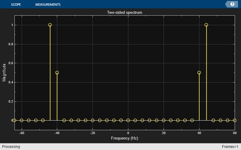
Compute the FFT of x and plot the magnitude of the FFT. The two sine waves are in adjacent samples of the FFT, which means that you cannot discriminate between frequencies closer than .
X = fft(x);
scopeFFT = dsp.ArrayPlot(SampleIncrement=Fs/L, ...
    XOffset=-Fs/2, ...
    XLabel="Frequency (Hz)", ...
    YLabel="Magnitude", ...
    Title="Two-sided spectrum", ...
    YLimits=[-0.1 1.1]);
scopeFFT(abs(fftshift(X))/L);
Zoom FFT
Suppose you have an application for which you are interested only in a sub-band of the Nyquist interval. The idea behind zoom FFT is to retain the same resolution you would achieve with a full size FFT on your original signal by computing a small FFT on a shorter signal. The shorter signal comes from decimating the original signal. The savings come from being able to compute a much shorter FFT while achieving the same resolution. For a decimation factor of D, the new sampling rate is , and the new frame size (and FFT length) is , so the resolution of the decimated signal is .
Mixer Approach
The mixer approach is a popular zoom FFT method.
Assume that you are interested only in the bandwidth interval of [16 Hz, 48 Hz] and calculate the center frequency of that interval.
BWOfInterest = 48 - 16;
Fc           = (16 + 48)/2; % Center frequency of bandwidth of interest
Calculate the achievable decimation factor using the sample rate from the example in the previous section.
BWFactor = floor(Fs/BWOfInterest)
BWFactor =
4
The mixer approach consists of first shifting the band of interest down to DC using a mixer, followed by lowpass filtering and decimation by a factor of BWFactor.
Design the coefficients of the decimation filter using the designMultirateFIR function. The returned dsp.FIRDecimator System object implements the lowpass and downsampling operations using an efficient polyphase FIR decimation structure.
D = designMultirateFIR(DecimationFactor=BWFactor,SystemObject=true);
Mix the signal down to DC, and filter it through the FIR decimator.
% Run several input frames to eliminate the FIR transient response
for k = 1:10
    % Grab a frame of the input signal
    x = sn1()+sn2();

    % Downmix to DC
    indVect = (0:numel(x)-1).' + (k-1) * size(x,1);
    y = x .* exp(-2*pi*indVect*Fc*1j/Fs);

    % Filter through FIR decimator
    xd = D(y);
end
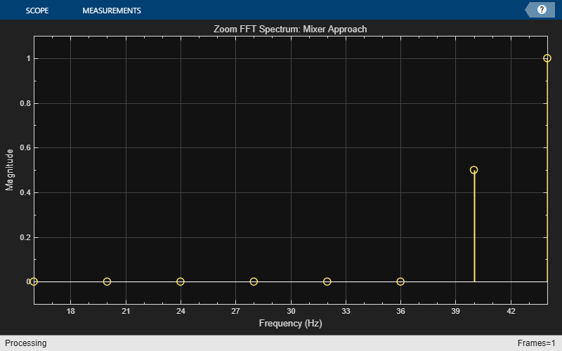
Compute the FFT of the filtered signal. To maintain the same resolution, the FFT length in the mixer approach reduces by BWFactor or decimation length compared to the FFT length in the regular FFT transformation.
Xd  = fft(xd);
Ld  = L/BWFactor;
Fsd = Fs/BWFactor;

scopeMixing = dsp.ArrayPlot(SampleIncrement=Fs/L, ...
    XOffset=Fsd/2, ...
    XLabel="Frequency (Hz)", ...
    YLabel="Magnitude", ...
    Title="Zoom FFT Spectrum: Mixer Approach", ...
    YLimits=[-0.1 1.1]);

scopeMixing(abs(fftshift(Xd))/Ld);
The complex-valued mixer adds an extra multiplication operation for each high-rate sample, which is not efficient. The next section presents an alternative, more efficient, zoom FFT approach.
Bandpass Sampling
An alternative zoom FFT method takes advantage of a known result from bandpass filtering (also sometimes called under-sampling): Assume that you are interested in the band of a signal with the sampling rate . If you pass the signal through a complex (one-sided) bandpass filter centered at with the bandwidth , and then downsample it by a factor of , you bring down the desired band to the baseband.
In general, if you cannot express in the form (where k is an integer), then the shifted, decimated spectrum will not be centered at DC. In fact, the center frequency Fc translates to [2]:
In this case, you can use a mixer (running at the low sample rate of the decimated signal) to center the desired band to zero Hertz.
Using the example from the previous section, obtain the coefficients of the complex bandpass filter by modulating the coefficients of the designed lowpass filter.
N   = length(D.Numerator);
numbp = D.Numerator .*exp(1j*(Fc / Fs)*2*pi*(0:N-1));
Dbp = dsp.FIRDecimator(BWFactor, numbp);
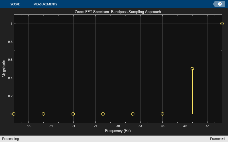
Perform the filtering and FFT operations.
for k = 1:10
    % Run a few times to eliminate transient in filter
    x = sn1()+sn2();
    xd = Dbp(x);
end
Xd = fft(xd);
scopeBandpassSampling = dsp.ArrayPlot(SampleIncrement=Fs/L, ...
                            XOffset=Fsd/2, ...
                            XLabel="Frequency (Hz)", ...
                            YLabel="Magnitude", ...
                            Title="Zoom FFT Spectrum: Bandpass Sampling Approach", ...
                            YLimits=[-0.1 1.1]);
scopeBandpassSampling(abs(fftshift(Xd))/Ld);
Multirate Multistage Bandpass Filter
The FIR decimator in the previous section is a single-stage multirate filter. You can reduce the computational complexity of the filter by using a multistage design instead (in fact, this is the approach utilized in dsp.ZoomFFT System Object). See Multistage Rate Conversion for more details.
Consider the following example, where the input sample rate is 48 KHz, and the bandwidth of interest is the interval [1500,2500] Hz. The achievable decimation factor is then .
First, design a single-stage decimator with a transition width of 1% of the Nyquist frequency.
Fs       = 48e3;
Fc       = 2000; % Bandpass filter center frequency
BW       = 1e3;  % Bandwidth of interest
Ast      = 80;   % Stopband attenuation
BWFactor = floor(Fs/BW);
TW       = 0.01;
B        = designMultirateFIR(DecimationFactor=BWFactor,...
                            TransitionWidth=TW,...
                            StopbandAttenuation=Ast);

N        = length(B);
Bbp      = B.*exp(1j*(Fc / Fs)*2*pi*(0:N-1));
D_single_stage = dsp.FIRDecimator(BWFactor, Bbp);
Now, implement the same decimator using a multistage design, while maintaining the same stopband attenuation and bandwidth as the single-stage case. You can calculate the input bandwidth by subtracting half the transition width from the cutoff frequency of the decimator filter.
Fcd = 1/BWFactor;        % Decimation passband cutoff frequency
BWNormalized = Fcd-TW/2; % Normalized input bandwidth
D_multi_stage = designRateConverter(DecimationFactor=BWFactor, ...
                                    InputSampleRate=Fs, ...
                                    Bandwidth = BWNormalized*(Fs/2), ...
                                    StopbandAttenuation=Ast);
fprintf("Number of filter stages: %d\n", getNumStages(D_multi_stage) );
Number of filter stages: 5
for ns=1:D_multi_stage.getNumStages
    stgn = D_multi_stage.("Stage" + ns);
    fprintf("Stage %i: Decimation factor = %d , FIR length = %d\n",...
            ns, stgn.DecimationFactor,...
            length(stgn.Numerator));
end
Stage 1: Decimation factor = 2 , FIR length = 7
Stage 2: Decimation factor = 2 , FIR length = 7
Stage 3: Decimation factor = 2 , FIR length = 11
Stage 4: Decimation factor = 2 , FIR length = 15
Stage 5: Decimation factor = 3 , FIR length = 59
This filter is a five-stage multirate lowpass filter. Transform it to a bandpass filter by performing a frequency shift on the coefficients of each stage, while taking the cumulative decimation factor into account.
Mn = 1; % Cumulative decimation factor entring stage n
for ns=1:D_multi_stage.getNumStages
    stgn = D_multi_stage.("Stage" + ns);
    num  = stgn.Numerator;
    N    = length(num);
    num  = num .*exp(1j*(Fc * Mn/ Fs)*2*pi*(0:N-1));
    stgn.Numerator = num;
    Mn   = Mn*stgn.DecimationFactor;
end
Calculate the cost of the single-stage filter.
cost(D_single_stage)
ans = struct with fields:
                  NumCoefficients: 985
                        NumStates: 960
    MultiplicationsPerInputSample: 20.5208
          AdditionsPerInputSample: 20.5000
Calculate the cost of the multistage filter. This filter is significantly more efficient computationally.
cost(D_multi_stage)
ans = struct with fields:
                  NumCoefficients: 67
                        NumStates: 93
    MultiplicationsPerInputSample: 6.0417
          AdditionsPerInputSample: 5.0833
Next, compare the frequency response of the two filters, and verify that the two filters have the same passband characteristics. The differences in the stopband are negligible.
FA = filterAnalyzer(D_single_stage,D_multi_stage,FrequencyRange="centered");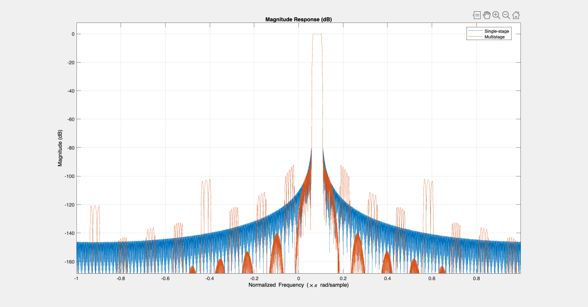
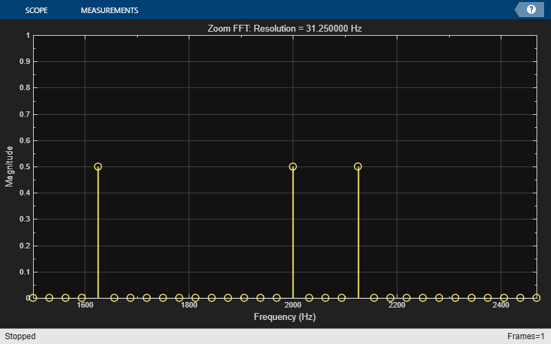
Finally, use the multistage filter to perform zoom FFT:
fftlen = 32;
L      = BWFactor * fftlen;
tones  = [1625 2000 2125]; % sine wave tones
sn     = dsp.SineWave(SampleRate=Fs, Frequency=tones, SamplesPerFrame=L);
Fsd    = Fs / BWFactor;
F      = Fc + Fsd/fftlen*(0:fftlen-1)-Fsd/2; % Discrete frequency points

% Step through the bandpass-decimator
for k=1:100
    x = sum(sn(),2) +  1e-2 * randn(L,1);
    y = D_multi_stage(x);
end

% Plot the spectral output
scopeZoomFFT = dsp.ArrayPlot(XDataMode="Custom",...
                   CustomXData=F,...
                   YLabel="Magnitude",...
                   XLabel="Frequency (Hz)",...
                   YLimits=[0 1],...
                   Title=sprintf ("Zoom FFT: Resolution = %f Hz",(Fs/BWFactor)/fftlen));

z = fft(y,fftlen,1);
z = fftshift(z);

scopeZoomFFT( abs(z)/fftlen )
release(scopeZoomFFT)
Using dsp.ZoomFFT
The dsp.ZoomFFT System object implements zoom FFT based on the multirate multistage bandpass filter described in the previous section. You specify the desired center frequency and decimation factor, and dsp.ZoomFFT designs the filter and applies it to the input signal.
Use dsp.ZoomFFT to zoom into the sine tones from the signal in the previous section.
zfft = dsp.ZoomFFT(BWFactor,Fc,Fs);
for k=1:100
    x = sum(sn(),2) + 1e-2 * randn(L,1);
    z = zfft(x);
end

z = fftshift(z);
scopeZoomFFT( abs(z)/fftlen)

release(scopeZoomFFT)

References
[1] Multirate Signal Processing - Harris (Prentice Hall).
[2] Computing Translated Frequencies in digitizing and Downsampling Analog Bandpass - Lyons (https://www.dsprelated.com/showarticle/523.php)
See Also
dsp.ZoomFFT | Zoom FFT | designMultirateFIR