Minimax FIR Filter Design

This example shows how to use some of the key features of the generalized Remez FIR filter design function. This function provides all the functionality included in firpm plus many additional features showcased here.

Weighted-Chebyshev Design

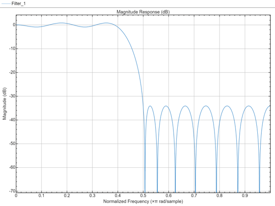
The following is an illustration of the weighted-Chebyshev design. This example shows the compatibility of firgr with firpm.

N = 22;             % Filter order
F = [0 0.4 0.5 1];  % Frequency vector
A = [1 1 0 0];      % Magnitude vector
W = [1 5];          % Weight vector
b = firgr(N,F,A,W);
filterAnalyzer(b,1)

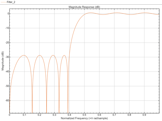
The following is a weighted-Chebyshev design where a type 4 filter (odd-order, asymmetric) has been explicitly specified.

N = 21;             % Filter order
F = [0 0.4 0.5 1];  % Frequency vector
A = [0 0 1 1];      % Magnitude vector
W = [2 1];          % Weight vector
b = firgr(N,F,A,W,'4');
filterAnalyzer(b,1)

"Least-Squares-Like" Design

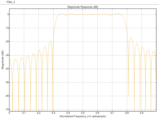
The following illustrates a "least-squares-like" design. A user-supplied frequency-response function (taperedresp.m) is used to perform the error weighting.

N = 53;                                  % Filter order
F = [0 0.3 0.33 0.77 0.8 1];             % Frequency vector
fresp = {@taperedresp, [0 0 1 1 0 0]};  % Frequency response function
W = [2 2 1];                             % Weight vector
b = firgr(N,F,fresp,W);
filterAnalyzer(b,1)

Filter Designed for Specific Single-Point Bands

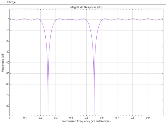
This is an illustration of a filter designed for specified single-point bands. The frequency points f = 0.25 and f = 0.55 are single-band points. These points have a gain that approaches zero.

The other band edges are normal.

N = 42;                               % Filter order
F = [0 0.2 0.25 0.3 0.5 0.55 0.6 1];  % Frequency vector
A = [1 1 0 1 1 0 1 1];                % Magnitude vector
S = {'n' 'n' 's' 'n' 'n' 's' 'n' 'n'};
b = firgr(N,F,A,S);
filterAnalyzer(b,1)

Filter Designed for Specific In-Band Value

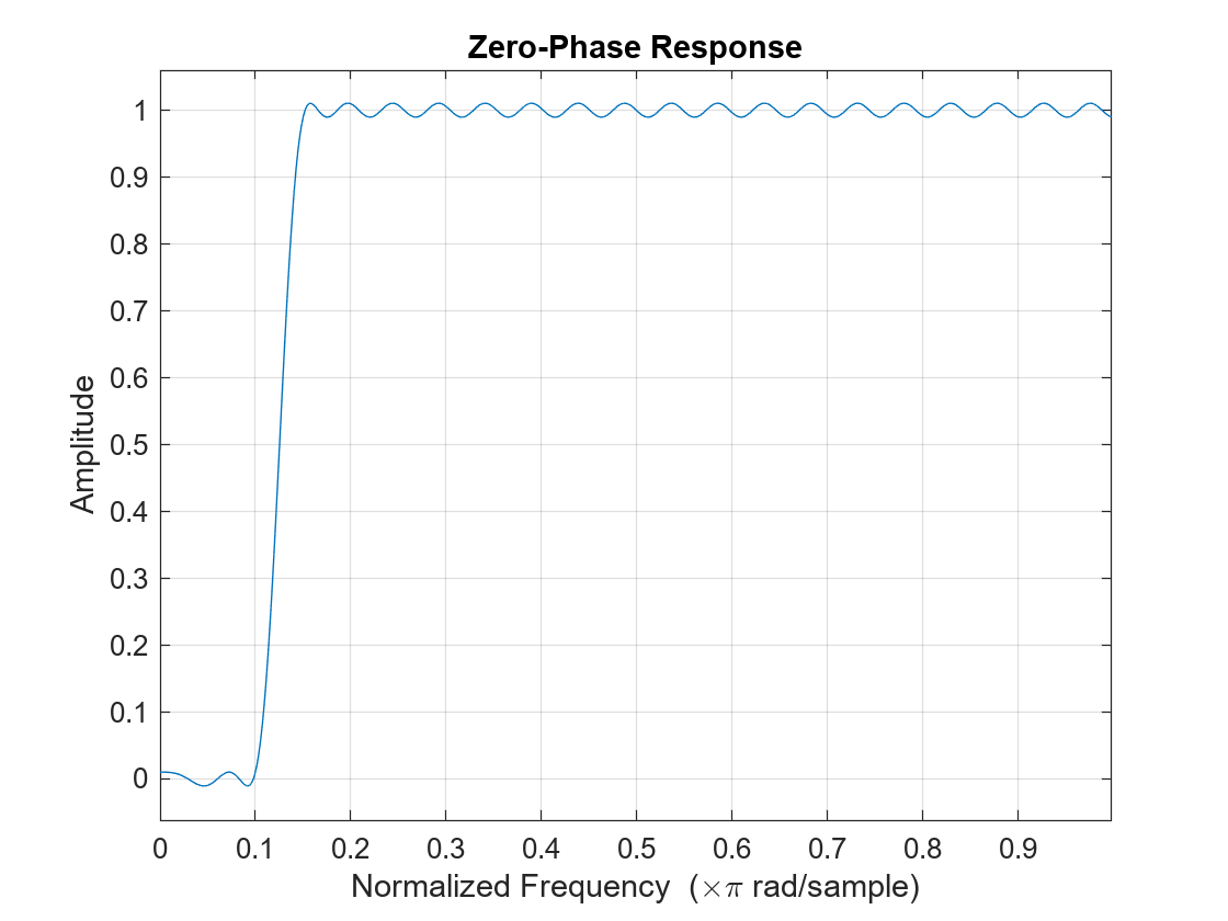
Here is an illustration of a filter designed for an exactly specified in-band value. The value is forced to be exactly the specified value of 0.0 at f = 0.06.

This could be used for 60 Hz rejection (with Fs = 2 kHz). The band edge at 0.055 is indeterminate since it should abut the next band.

N = 82;                         % Filter order
F = [0 0.055 0.06 0.1 0.15 1];  % Frequency vector
A = [0 0 0 0 1 1];              % Magnitude vector
S = {'n' 'i' 'f' 'n' 'n' 'n'};
b = firgr(N,F,A,S);
zerophase(b,1)

Filter Design with Specific Multiple Independent Approximation Errors

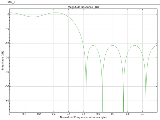
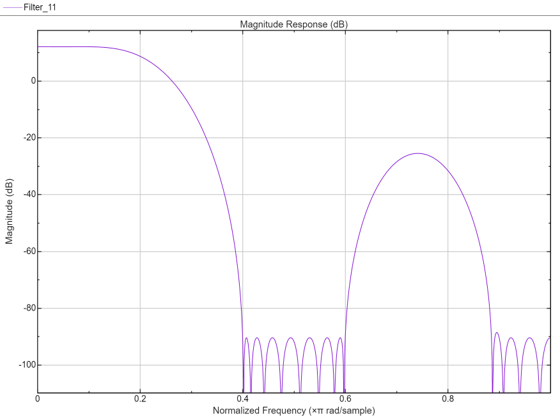
Here is an example of designing a filter using multiple independent approximation errors. This technique is used to directly design extra-ripple and maximal ripple filters. One of the interesting properties that these filters have is a transition region width that is locally minimal. Further, these designs converge very quickly in general.

N = 12;             % Filter order
F = [0 0.4 0.5 1];  % Frequency vector
A = [1 1 0 0];      % Magnitude vector
W = [1 1];          % Weight vector
E = {'e1' 'e2'};    % Approximation errors
b = firgr(N,F,A,W,E);
filterAnalyzer(b,1)

Extra-Ripple Bandpass Filter

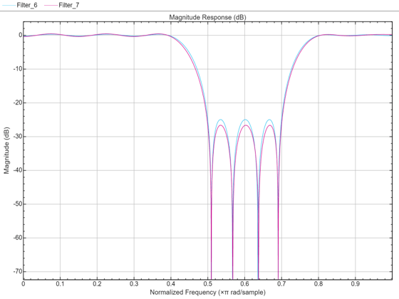
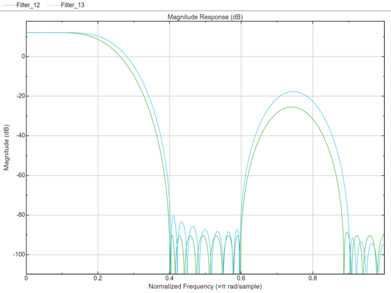
Here is an illustration of an extra-ripple bandpass filter having two independent approximation errors: one shared by the two passbands and the other for the stopband (in blue). For comparison, a standard weighted-Chebyshev design is also plotted (in green).

N = 28;                     % Filter order
F = [0 0.4 0.5 0.7 0.8 1];  % Frequency vector
A = [1 1 0 0 1 1];          % Magnitude vector
W = [1 1 2];                % Weight vector
E = {'e1','e2','e1'};       % Approximation errors
b1 = firgr(N,F,A,W,E);
b2 = firgr(N,F,A,W);
filterAnalyzer(b1,1,b2,1)

Designing an In-Band-Zero Filter Using Three Independent Errors

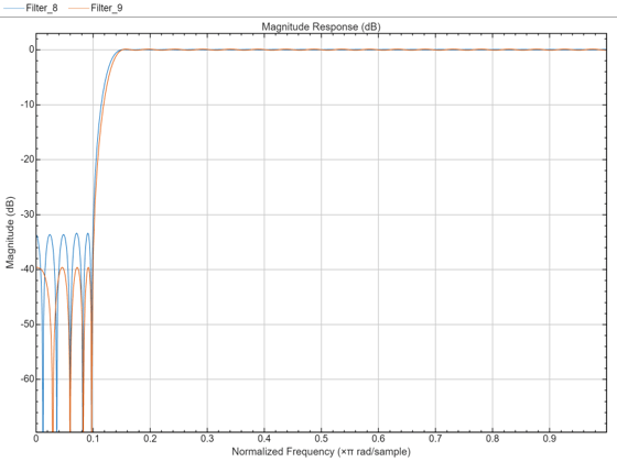
We'll now re-do our in-band-zero example using three independent errors.

Note: It is sometimes necessary to use independent approximation errors to get designs with forced in-band values to converge. This is because the approximating polynomial could otherwise be come very underdetermined. The former design is displayed in green.

N = 82;                         % Filter order
F = [0 0.055 0.06 0.1 0.15 1];  % Frequency vector
A = [0 0 0 0 1 1];              % Magnitude vector
S = {'n' 'i' 'f' 'n' 'n' 'n'};
W = [10 1 1];                   % Weight vector
E = {'e1' 'e2' 'e3'};           % Approximation errors
b1 = firgr(N,F,A,S,W,E);
b2 = firgr(N,F,A,S);
filterAnalyzer(b1,1,b2,1)

Checking for Transition-Region Anomalies

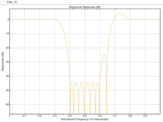
With the 'check' option, one is made aware of possible transition region anomalies in the filter that is being designed. Here is an example of a filter with an anomaly. The 'check' option warns one of this anomaly: One also get a results vector res.edgeCheck. Any zero-valued elements in this vector indicate the locations of probable anomalies. The "-1" entries are for edges that were not checked (there can't be an anomaly at f = 0 or f = 1).

N = 44;                     % Filter order
F = [0 0.3 0.4 0.6 0.8 1];  % Frequency vector
A = [1 1 0 0 1 1];          % Magnitude vector
b = firgr(N,F,A,'check');

Warning: Probable transition-region anomalies.  Verify with freqz.

filterAnalyzer(b,1)

Determination of the Minimum Filter Order

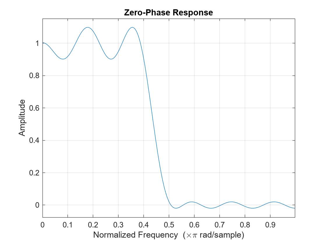
The firpm algorithm repeatedly designs filters until the first iteration wherein the specifications are met. The specifications are met when all of the required constraints are met. By specifying 'minorder', firpmord is used to get an initial estimate. There is also 'mineven' and 'minodd' to get the minimum-order even-order or odd-order filter designs.

F = [0 0.4 0.5 1];  % Frequency vector
A = [1 1 0 0];      % Magnitude vector
R = [0.1 0.02];     % Deviation (ripple) vector
b = firgr('minorder',F,A,R);
zerophase(b,1)

Differentiators and Hilbert Transformers

While using the minimum-order feature, an initial estimate of the filter order can be made. If this is the case, then firpmord will not be used. This is necessary for filters that firpmord does not support, such as differentiators and Hilbert transformers as well as user-supplied frequency-response functions.

N = {'mineven',18}; % Minimum even-order, start order estimate at 18
F = [0.1 0.9];      % Frequency vector
A = [1 1];          % Magnitude vector
R = 0.1;            % Deviation (ripple)
b = firgr(N,F,A,R,'hilbert');
freqz(b,1,'whole')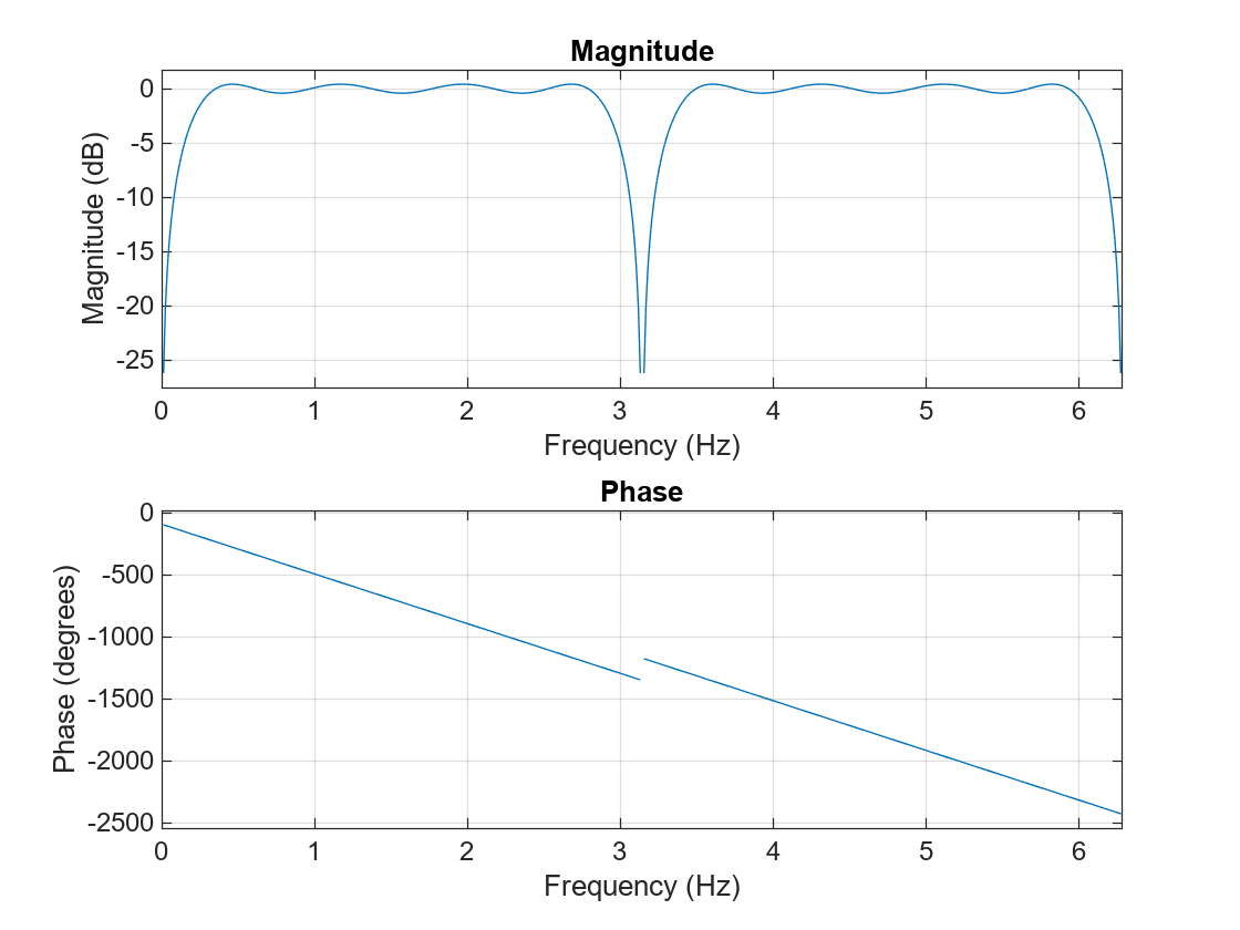

Design of an Interpolation Filter

This section illustrates the use of an interpolation filter for upsampling band-limited signals by an integer factor. Typically one would use intfilt(r,l,alpha) from the Signal Processing Toolbox™ to do this. However, intfilt does not give one as much flexibility in the design as does firgr.

N = 30;                     % Filter order
F = [0 0.1 0.4 0.6 0.9 1];  % Frequency vector
A = [4 4 0 0 0 0];          % Magnitude vector
W = [1 100 100];            % Weight vector
b = firgr(N,F,A,W);
filterAnalyzer(b,1)

A Comparison Between firpm and intfilt

Here is a comparison made between a filter designed using firpm (blue) and a 30-th order filter designed using intfilt (green).

Notice that by using the weighting function in firpm, one can improve the minimum stopband attenuation by almost 20 dB.

b2 = intfilt(4, 4, 0.4);
filterAnalyzer(b,1,b2,1)

Notice that the equiripple attenuation throughout the second stopband is larger than the minimum stopband attenuation of the filter designed with intfilt by about 6 dB. Notice also that the passband ripple, although larger than that of the filter designed with intfilt, is still very small.

Design of a Minimum-Phase Lowpass Filter

Here is an illustration of a minimum-phase lowpass filter.

N = 42;             % Filter order
F = [0 0.4 0.5 1];  % Frequency vector
A = [1 1 0 0];      % Magnitude vector
W = [1 10];        % Weight-constraint vector
b = firgr(N,F,A,W, {64},'minphase');

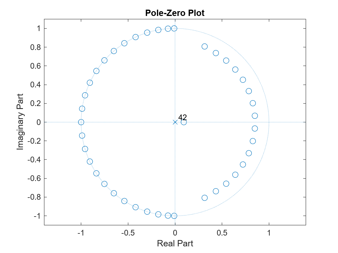
The pole/zero plot shows that there are no roots outside of the unit circle.

zplane(b,1)