Visual-Inertial Odometry Using Synthetic Data
This example shows how to estimate the pose (position and orientation) of a ground vehicle using an inertial measurement unit (IMU) and a monocular camera. In this example, you:
Create a driving scenario containing the ground truth trajectory of the vehicle.
Use an IMU and visual odometry model to generate measurements.
Fuse these measurements to estimate the pose of the vehicle and then display the results.
Visual-inertial odometry estimates pose by fusing the visual odometry pose estimate from the monocular camera and the pose estimate from the IMU. The IMU returns an accurate pose estimate for small time intervals, but suffers from large drift due to integrating the inertial sensor measurements. The monocular camera returns an accurate pose estimate over a larger time interval, but suffers from a scale ambiguity. Given these complementary strengths and weaknesses, the fusion of these sensors using visual-inertial odometry is a suitable choice. This method can be used in scenarios where GPS readings are unavailable, such as in an urban canyon.
Create a Driving Scenario with Trajectory
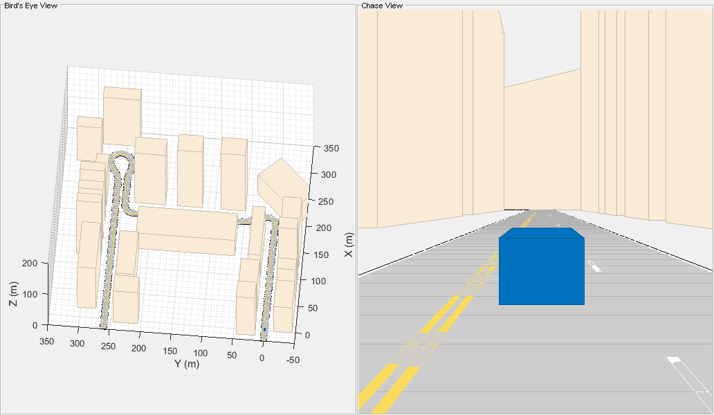
Create a drivingScenario object that contains:
The road the vehicle travels on
The buildings surrounding either side of the road
The ground truth pose of the vehicle
The estimated pose of the vehicle
The ground truth pose of the vehicle is shown as a solid blue cuboid. The estimated pose is shown as a transparent blue cuboid. Note that the estimated pose does not appear in the initial visualization because the ground truth and estimated poses overlap.
Generate the baseline trajectory for the ground vehicle using the waypointTrajectory (Sensor Fusion and Tracking Toolbox) System object™. Note that the waypointTrajectory is used in place of drivingScenario/trajectory since the acceleration of the vehicle is needed. The trajectory is generated at a specified sampling rate using a set of waypoints, times of arrival, and velocities.
% Create the driving scenario with both the ground truth and estimated
% vehicle poses.
scene = drivingScenario;
groundTruthVehicle = vehicle(scene, 'PlotColor', [0 0.4470 0.7410]);
estVehicle = vehicle(scene, 'PlotColor', [0 0.4470 0.7410]);

% Generate the baseline trajectory.
sampleRate = 100;
wayPoints = [  0   0 0;
             200   0 0;
             200  50 0;
             200 230 0;
             215 245 0;
             260 245 0;
             290 240 0;
             310 258 0;
             290 275 0;
             260 260 0;
             -20 260 0];
t = [0 20 25 44 46 50 54 56 59 63 90].';
speed = 10;
velocities = [ speed     0 0;
               speed     0 0;
                   0 speed 0;
                   0 speed 0;
               speed     0 0;
               speed     0 0;
               speed     0 0;
                   0 speed 0;
              -speed     0 0;
              -speed     0 0;
              -speed     0 0];

traj = waypointTrajectory(wayPoints, 'TimeOfArrival', t, ...
    'Velocities', velocities, 'SampleRate', sampleRate);

% Add a road and buildings to scene and visualize.
helperPopulateScene(scene, groundTruthVehicle);

Create a Fusion Filter
Create the filter to fuse IMU and visual odometry measurements. This example uses a loosely coupled method to fuse the measurements. While the results are not as accurate as a tightly coupled method, the amount of processing required is significantly less and the results are adequate. The fusion filter uses an error-state Kalman filter to track orientation (as a quaternion), position, velocity, and sensor biases.
The insfilterErrorState object has the following functions to process sensor data: predict and fusemvo.
The predict function takes the accelerometer and gyroscope measurements from the IMU as inputs. Call the predict function each time the accelerometer and gyroscope are sampled. This function predicts the state forward by one time step based on the accelerometer and gyroscope measurements, and updates the error state covariance of the filter.
The fusemvo function takes the visual odometry pose estimates as input. This function updates the error states based on the visual odometry pose estimates by computing a Kalman gain that weighs the various inputs according to their uncertainty. As with the predict function, this function also updates the error state covariance, this time taking the Kalman gain into account. The state is then updated using the new error state and the error state is reset.
filt = insfilterErrorState('IMUSampleRate', sampleRate, ...
    'ReferenceFrame', 'ENU')
% Set the initial state and error state covariance.
helperInitialize(filt, traj);
filt =

  insfilterErrorState with properties:

        IMUSampleRate: 100               Hz
    ReferenceLocation: [0 0 0]           [deg deg m]
                State: [17⨯1 double]
      StateCovariance: [16⨯16 double]

   Process Noise Variances
            GyroscopeNoise: [1e-06 1e-06 1e-06]       (rad/s)²
        AccelerometerNoise: [0.0001 0.0001 0.0001]    (m/s²)²
        GyroscopeBiasNoise: [1e-09 1e-09 1e-09]       (rad/s)²
    AccelerometerBiasNoise: [0.0001 0.0001 0.0001]    (m/s²)²
Specify the Visual Odometry Model
Define the visual odometry model parameters. These parameters model a feature matching and tracking-based visual odometry system using a monocular camera. The scale parameter accounts for the unknown scale of subsequent vision frames of the monocular camera. The other parameters model the drift in the visual odometry reading as a combination of white noise and a first-order Gauss-Markov process.
% The flag useVO determines if visual odometry is used:
% useVO = false; % Only IMU is used.
useVO = true; % Both IMU and visual odometry are used.

paramsVO.scale = 2;
paramsVO.sigmaN = 0.139;
paramsVO.tau = 232;
paramsVO.sigmaB = sqrt(1.34);
paramsVO.driftBias = [0 0 0];
Specify the IMU Sensor
Define an IMU sensor model containing an accelerometer and gyroscope using the imuSensor System object. The sensor model contains properties to model both deterministic and stochastic noise sources. The property values set here are typical for low-cost MEMS sensors.
% Set the RNG seed to default to obtain the same results for subsequent
% runs.
rng('default')

imu = imuSensor('SampleRate', sampleRate, 'ReferenceFrame', 'ENU');

% Accelerometer
imu.Accelerometer.MeasurementRange =  19.6; % m/s^2
imu.Accelerometer.Resolution = 0.0024; % m/s^2/LSB
imu.Accelerometer.NoiseDensity = 0.01; % (m/s^2)/sqrt(Hz)

% Gyroscope
imu.Gyroscope.MeasurementRange = deg2rad(250); % rad/s
imu.Gyroscope.Resolution = deg2rad(0.0625); % rad/s/LSB
imu.Gyroscope.NoiseDensity = deg2rad(0.0573); % (rad/s)/sqrt(Hz)
imu.Gyroscope.ConstantBias = deg2rad(2); % rad/s
Set Up the Simulation
Specify the amount of time to run the simulation and initialize variables that are logged during the simulation loop.
% Run the simulation for 60 seconds.
numSecondsToSimulate = 60;
numIMUSamples = numSecondsToSimulate * sampleRate;

% Define the visual odometry sampling rate.
imuSamplesPerCamera = 4;
numCameraSamples = ceil(numIMUSamples / imuSamplesPerCamera);

% Preallocate data arrays for plotting results.
[pos, orient, vel, acc, angvel, ...
    posVO, orientVO, ...
    posEst, orientEst, velEst] ...
    = helperPreallocateData(numIMUSamples, numCameraSamples);

% Set measurement noise parameters for the visual odometry fusion.
RposVO = 0.1;
RorientVO = 0.1;
Run the Simulation Loop
Run the simulation at the IMU sampling rate. Each IMU sample is used to predict the filter's state forward by one time step. Once a new visual odometry reading is available, it is used to correct the current filter state.
There is some drift in the filter estimates that can be further corrected with an additional sensor such as a GPS or an additional constraint such as a road boundary map.
cameraIdx = 1;
for i = 1:numIMUSamples
    % Generate ground truth trajectory values.
    [pos(i,:), orient(i,:), vel(i,:), acc(i,:), angvel(i,:)] = traj();

    % Generate accelerometer and gyroscope measurements from the ground truth
    % trajectory values.
    [accelMeas, gyroMeas] = imu(acc(i,:), angvel(i,:), orient(i));

    % Predict the filter state forward one time step based on the
    % accelerometer and gyroscope measurements.
    predict(filt, accelMeas, gyroMeas);

    if (1 == mod(i, imuSamplesPerCamera)) && useVO
        % Generate a visual odometry pose estimate from the ground truth
        % values and the visual odometry model.
        [posVO(cameraIdx,:), orientVO(cameraIdx,:), paramsVO] = ...
            helperVisualOdometryModel(pos(i,:), orient(i,:), paramsVO);

        % Correct filter state based on visual odometry data.
        fusemvo(filt, posVO(cameraIdx,:), RposVO, ...
            orientVO(cameraIdx), RorientVO);

        cameraIdx = cameraIdx + 1;
    end

    [posEst(i,:), orientEst(i,:), velEst(i,:)] = pose(filt);

    % Update estimated vehicle pose.
    helperUpdatePose(estVehicle, posEst(i,:), velEst(i,:), orientEst(i));

    % Update ground truth vehicle pose.
    helperUpdatePose(groundTruthVehicle, pos(i,:), vel(i,:), orient(i));

    % Update driving scenario visualization.
    updatePlots(scene);
    drawnow limitrate;
end

Plot the Results
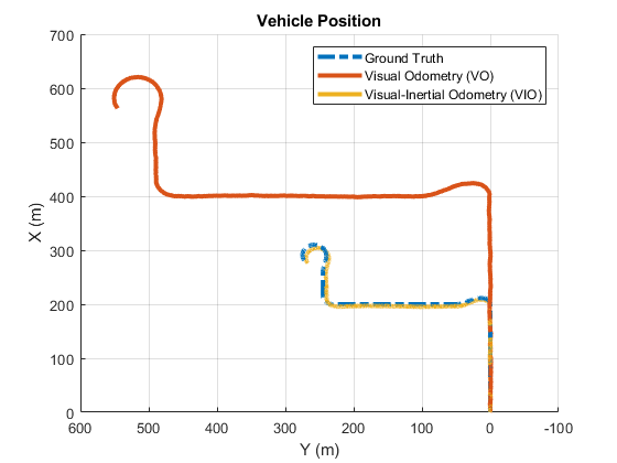
Plot the ground truth vehicle trajectory, the visual odometry estimate, and the fusion filter estimate.
figure
if useVO
    plot3(pos(:,1), pos(:,2), pos(:,3), '-.', ...
        posVO(:,1), posVO(:,2), posVO(:,3), ...
        posEst(:,1), posEst(:,2), posEst(:,3), ...
        'LineWidth', 3)
    legend('Ground Truth', 'Visual Odometry (VO)', ...
        'Visual-Inertial Odometry (VIO)', 'Location', 'northeast')
else
    plot3(pos(:,1), pos(:,2), pos(:,3), '-.', ...
        posEst(:,1), posEst(:,2), posEst(:,3), ...
        'LineWidth', 3)
    legend('Ground Truth', 'IMU Pose Estimate')
end
view(-90, 90)
title('Vehicle Position')
xlabel('X (m)')
ylabel('Y (m)')
grid on

The plot shows that the visual odometry estimate is relatively accurate in estimating the shape of the trajectory. The fusion of the IMU and visual odometry measurements removes the scale factor uncertainty from the visual odometry measurements and the drift from the IMU measurements.
Supporting Functions
helperVisualOdometryModel
Compute visual odometry measurement from ground truth input and parameters struct. To model the uncertainty in the scaling between subsequent frames of the monocular camera, a constant scaling factor combined with a random drift is applied to the ground truth position.
function [posVO, orientVO, paramsVO] ...
    = helperVisualOdometryModel(pos, orient, paramsVO)

% Extract model parameters.
scaleVO = paramsVO.scale;
sigmaN = paramsVO.sigmaN;
tau = paramsVO.tau;
sigmaB = paramsVO.sigmaB;
sigmaA = sqrt((2/tau) + 1/(tau*tau))*sigmaB;
b = paramsVO.driftBias;

% Calculate drift.
b = (1 - 1/tau).*b + randn(1,3)*sigmaA;
drift = randn(1,3)*sigmaN + b;
paramsVO.driftBias = b;

% Calculate visual odometry measurements.
posVO = scaleVO*pos + drift;
orientVO = orient;
end
helperInitialize
Set the initial state and covariance values for the fusion filter.
function helperInitialize(filt, traj)

% Retrieve the initial position, orientation, and velocity from the
% trajectory object and reset the internal states.
[pos, orient, vel] = traj();
reset(traj);

% Set the initial state values.
filt.State(1:4) = compact(orient(1)).';
filt.State(5:7) = pos(1,:).';
filt.State(8:10) = vel(1,:).';

% Set the gyroscope bias and visual odometry scale factor covariance to
% large values corresponding to low confidence.
filt.StateCovariance(10:12,10:12) = 1e6;
filt.StateCovariance(end) = 2e2;
end
helperPreallocateData
Preallocate data to log simulation results.
function [pos, orient, vel, acc, angvel, ...
    posVO, orientVO, ...
    posEst, orientEst, velEst] ...
    = helperPreallocateData(numIMUSamples, numCameraSamples)

% Specify ground truth.
pos = zeros(numIMUSamples, 3);
orient = quaternion.zeros(numIMUSamples, 1);
vel = zeros(numIMUSamples, 3);
acc = zeros(numIMUSamples, 3);
angvel = zeros(numIMUSamples, 3);

% Visual odometry output.
posVO = zeros(numCameraSamples, 3);
orientVO = quaternion.zeros(numCameraSamples, 1);

% Filter output.
posEst = zeros(numIMUSamples, 3);
orientEst = quaternion.zeros(numIMUSamples, 1);
velEst = zeros(numIMUSamples, 3);
end
helperUpdatePose
Update the pose of the vehicle.
function helperUpdatePose(veh, pos, vel, orient)

veh.Position = pos;
veh.Velocity = vel;
rpy = eulerd(orient, 'ZYX', 'frame');
veh.Yaw = rpy(1);
veh.Pitch = rpy(2);
veh.Roll = rpy(3);
end
References
Sola, J. "Quaternion Kinematics for the Error-State Kalman Filter." ArXiv e-prints, arXiv:1711.02508v1 [cs.RO] 3 Nov 2017.
R. Jiang, R., R. Klette, and S. Wang. "Modeling of Unbounded Long-Range Drift in Visual Odometry." 2010 Fourth Pacific-Rim Symposium on Image and Video Technology. Nov. 2010, pp. 121-126.
See Also
waypointTrajectory (Sensor Fusion and Tracking Toolbox) | imuSensor (Sensor Fusion and Tracking Toolbox) | drivingScenario