Velocity Profile of Straight Path
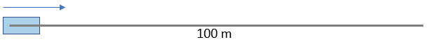
This model uses a Velocity Profiler block to generate a velocity profile for a vehicle traveling forward on a straight, 100-meter path that has no changes in direction.
The Velocity Profiler block generates velocity profiles based on the speed, acceleration, and jerk constraints that you specify using parameters. You can use the generated velocity profile as the input reference velocities of a vehicle controller.
This model is for illustrative purposes and does not show how to use the Velocity Profiler block in a complete automated driving model. To see how to use this block in such a model, see the Automated Parking Valet in Simulink example.
Open and Inspect Model
The model consists of a single Velocity Profiler block with constant inputs. Open the model.
model = 'VelocityProfileStraightPath';
open_system(model)
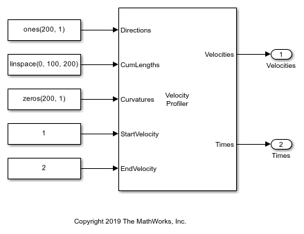
The first three inputs specify information about the driving path.
The Directions input specifies the driving direction of the vehicle along the path, where 1 means forward and –1 means reverse. Because the vehicle travels only forward, the direction is 1 along the entire path.
The CumLengths input specifies the length of the path. The path is 100 meters long and is composed of a sequence of 200 cumulative path lengths.
The Curvatures input specifies the curvature along the path. Because this path is straight, the curvature is 0 along the entire path.
In a complete automated driving model, you can obtain these input values from the output of a Path Smoother Spline block, which smooths a path based on a set of poses.
The StartVelocity and EndVelocity inputs specify the velocity of the vehicle at the start and end of the path, respectively. The vehicle starts the path traveling at a velocity of 1 meter per second and reaches the end of the path traveling at a velocity of 2 meters per second.
Generate Velocity Profile
Simulate the model to generate the velocity profile.
out = sim(model);
The output velocity profile is a sequence of velocities along the path that meet the speed, acceleration, and jerk constraints specified in the parameters of the Velocity Profiler block.
The block also outputs the times at which the vehicle arrives at each point along the path. You can use this output to visualize the velocities over time.
Visualize Velocity Profile
Use the simulation output to plot the velocity profile.
t = length(out.tout);
velocities = out.yout.signals(1).values(:,:,t);
times = out.yout.signals(2).values(:,:,t);

plot(times,velocities)
title('Velocity Profile')
xlabel('Times (s)')
ylabel('Velocities (m/s)')
grid on
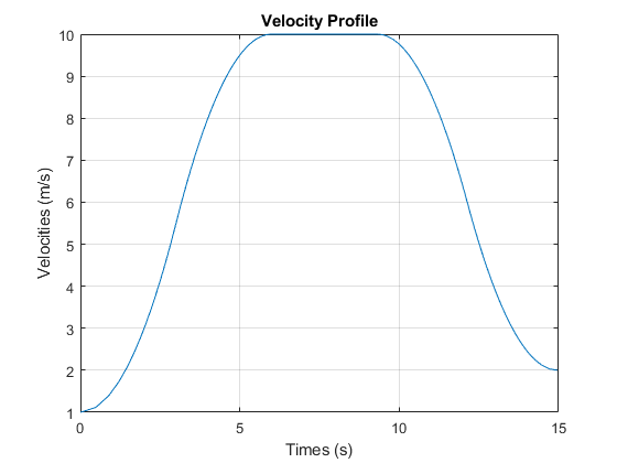
A vehicle that follows this velocity profile:
Starts at a velocity of 1 meter per second
Accelerates to a maximum speed of 10 meters per second, as specified by the Maximum allowable speed (m/s) parameter of the Velocity Profiler block
Decelerates to its ending velocity of 2 meters per second
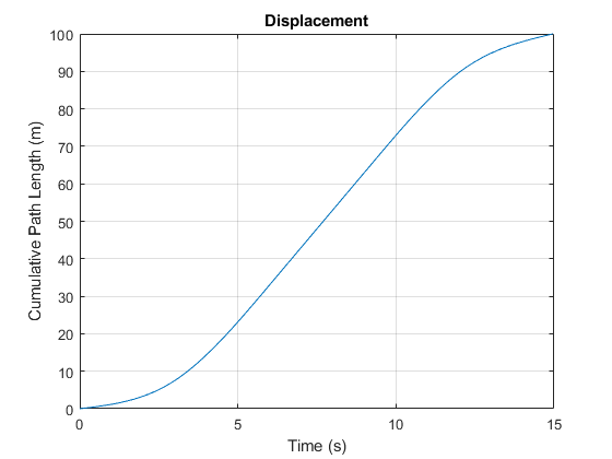
For comparison, plot the displacement of the vehicle over time by using the cumulative path lengths.
figure
cumLengths = linspace(0,100,200);
plot(times,cumLengths)
title('Displacement')
xlabel('Time (s)')
ylabel('Cumulative Path Length (m)')
grid on
For details on how the block calculates the velocity profile, see the Algorithms section of the Velocity Profiler block reference page.
See Also
Velocity Profiler | Path Smoother Spline