Fit Data Using the Neural Net Fitting App

This example shows how to train a shallow neural network to fit data using the Neural Net Fitting app.

Open the Neural Net Fitting app using nftool.

nftool

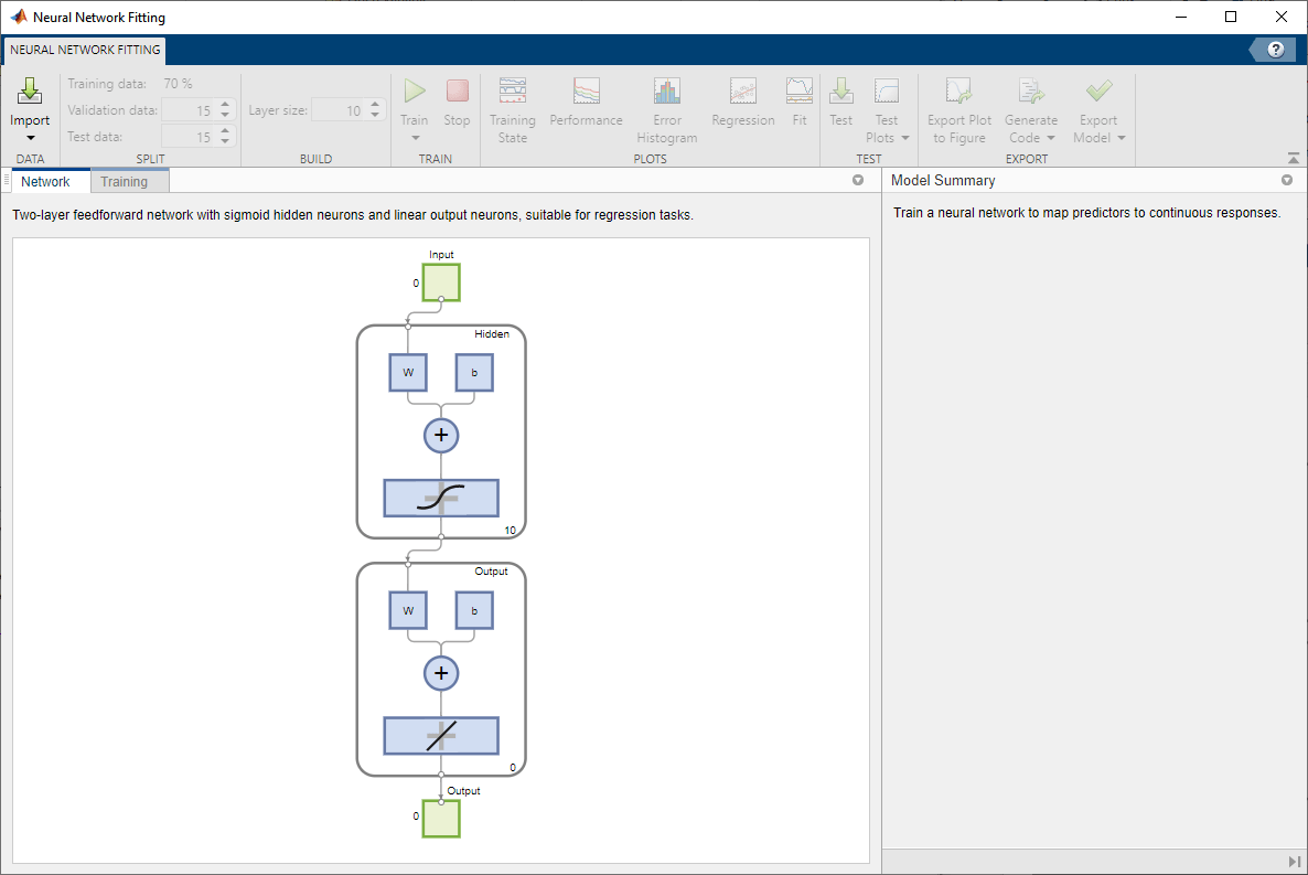
Select Data

The Neural Net Fitting app has example data to help you get started training a neural network.

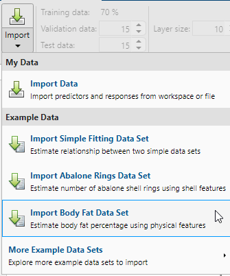
To import example body fat data, select Import > Import Body Fat Data Set. You can use this data set to train a neural network to estimate the body fat of someone from various measurements. If you import your own data from file or the workspace, you must specify the predictors and responses, and whether the observations are in rows or columns.

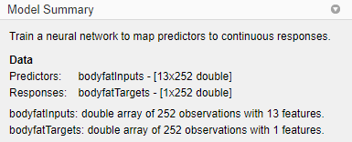
Information about the imported data appears in the Model Summary. This data set contains 252 observations, each with 13 features. The responses contain the body fat percentage for each observation.

Split the data into training, validation, and test sets. Keep the default settings. The data is split into:

• 70% for training.

• 15% to validate that the network is generalizing and to stop training before overfitting.

• 15% to independently test network generalization.

For more information on data division, see Divide Data for Optimal Neural Network Training.

Create Network

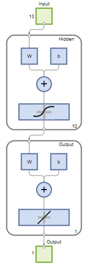
The network is a two-layer feedforward network with a sigmoid transfer function in the hidden layer and a linear transfer function in the output layer. The Layer size value defines the number of hidden neurons. Keep the default layer size, 10. You can see the network architecture in the Network pane. The network plot updates to reflect the input data. In this example, the data has 13 inputs (features) and one output.

Train Network

To train the network, select Train > Train with Levenberg-Marquardt. This is the default training algorithm and the same as clicking Train.

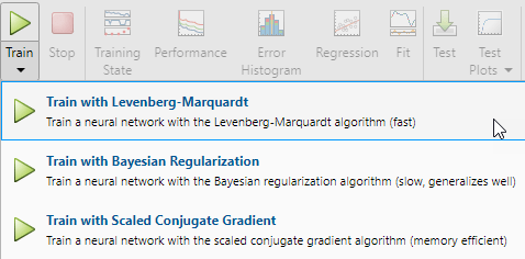
Training with Levenberg-Marquardt (trainlm) is recommended for most problems. For noisy or small problems, Bayesian Regularization (trainbr) can obtain a better solution, at the cost of taking longer. For large problems, Scaled Conjugate Gradient (trainscg) is recommended as it uses gradient calculations which are more memory efficient than the Jacobian calculations the other two algorithms use.

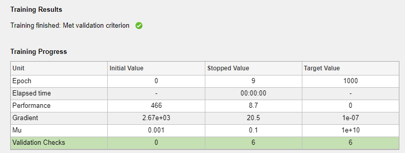
In the Training pane, you can see the training progress. Training continues until one of the stopping criteria is met. In this example, training continues until the validation error is larger than or equal to the previously smallest validation error for six consecutive validation iterations ("Met validation criterion").

Analyze Results

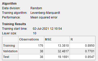
The Model Summary contains information about the training algorithm and the training results for each data set.

You can further analyze the results by generating plots. To plot the linear regression, in the Plots section, click Regression. The regression plot displays the network predictions (output) with respect to responses (target) for the training, validation, and test sets.

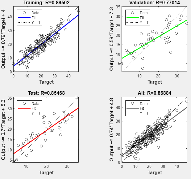
For a perfect fit, the data should fall along a 45 degree line, where the network outputs are equal to the responses. For this problem, the fit is reasonably good for all of the data sets. If you require more accurate results, you can retrain the network by clicking Train again. Each training will have different initial weights and biases of the network, and can produce an improved network after retraining.

View the error histogram to obtain additional verification of network performance. In the Plots section, click Error Histogram.

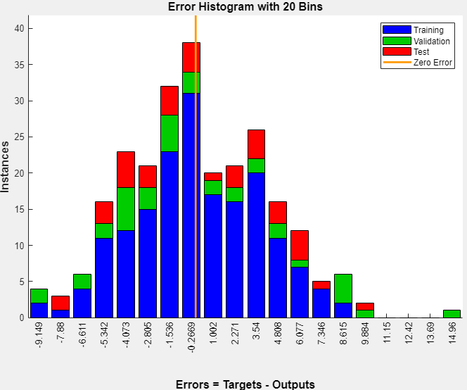
The blue bars represent training data, the green bars represent validation data, and the red bars represent testing data. The histogram provides an indication of outliers, which are data points where the fit is significantly worse than most of the data. It is a good idea to check the outliers to determine if the data is poor, or if those data points are different than the rest of the data set. If the outliers are valid data points, but are unlike the rest of the data, then the network is extrapolating for these points. You should collect more data that looks like the outlier points and retrain the network.

If you are unhappy with the network performance, you can do one of the following:

• Train the network again.

• Increase the number of hidden neurons.

• Use a larger training data set.

If performance on the training set is good but the test set performance is poor, this could indicate the model is overfitting. Reducing the number of neurons can reduce the overfitting.

You can also evaluate the network performance on an additional test set. To load additional test data to evaluate the network with, in the Test section, click Test. The Model Summary displays the additional test results. You can also generate plots to analyze the additional test data results.

Generate Code

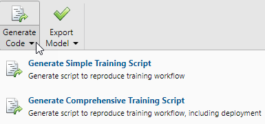
Select Generate Code > Generate Simple Training Script to create MATLAB code to reproduce the previous steps from the command line. Creating MATLAB code can be helpful if you want to learn how to use the command line functionality of the toolbox to customize the training process. In Fit Data Using Command-Line Functions, you will investigate the generated scripts in more detail.

Export Network

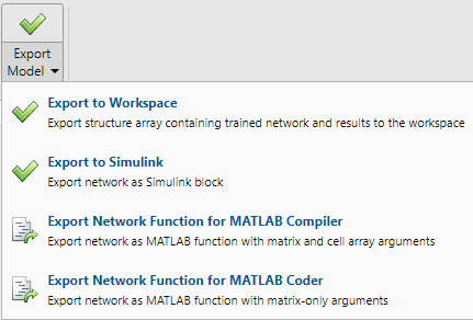
You can export your trained network to the workspace or Simulink®. You can also deploy the network with MATLAB Compiler™ tools and other MATLAB code generation tools. To export your trained network and results, select Export Model > Export to Workspace.