Convert Classification Network into Regression Network
This example shows how to convert a trained classification network into a regression network.
Pretrained image classification networks have been trained on over a million images and can classify images into 1000 object categories, such as keyboard, coffee mug, pencil, and many animals. The networks have learned rich feature representations for a wide range of images. The network takes an image as input, and then outputs a label for the object in the image together with the probabilities for each of the object categories.
Transfer learning is commonly used in deep learning applications. You can take a pretrained network and use it as a starting point to learn a new task. This example shows how to take a pretrained classification network and retrain it for regression tasks.
The example loads a pretrained convolutional neural network architecture for classification, replaces the layers for classification and retrains the network to predict angles of rotated handwritten digits.
Load Pretrained Network
Load the pretrained network from the supporting file digitsClassificationConvolutionNet.mat. This file contains a classification network that classifies handwritten digits.
load digitsClassificationConvolutionNet
layers = net.Layers
layers =
13×1 Layer array with layers:
1 'imageinput' Image Input 28×28×1 images
2 'conv_1' 2-D Convolution 10 3×3×1 convolutions with stride [2 2] and padding [0 0 0 0]
3 'batchnorm_1' Batch Normalization Batch normalization with 10 channels
4 'relu_1' ReLU ReLU
5 'conv_2' 2-D Convolution 20 3×3×10 convolutions with stride [2 2] and padding [0 0 0 0]
6 'batchnorm_2' Batch Normalization Batch normalization with 20 channels
7 'relu_2' ReLU ReLU
8 'conv_3' 2-D Convolution 40 3×3×20 convolutions with stride [2 2] and padding [0 0 0 0]
9 'batchnorm_3' Batch Normalization Batch normalization with 40 channels
10 'relu_3' ReLU ReLU
11 'gap' 2-D Global Average Pooling 2-D global average pooling
12 'fc' Fully Connected Fully connected layer with output size 10
13 'softmax' Softmax Softmax
Load Data
The data set contains synthetic images of handwritten digits together with the corresponding angles (in degrees) by which each image is rotated.
Load the training and test images as 4-D arrays from the supporting files DigitsDataTrain.mat and DigitsDataTest.mat. The variables anglesTrain and anglesTest are the rotation angles in degrees. The training and test data sets each contain 5000 images.
load DigitsDataTrain
load DigitsDataTest
Display 20 random training images using imshow.
numTrainImages = numel(anglesTrain);
figure
idx = randperm(numTrainImages,20);
for i = 1:numel(idx)
    subplot(4,5,i)
    imshow(XTrain(:,:,:,idx(i)))
end

Replace Final Layers
The convolutional layers of the network extract image features that the last learnable layer used to classify the input image. The layer "fc" contains the information on how to combine the features that the network extracts into class probabilities. To retrain a pretrained network for regression, replace this layer and the following softmax layer with a new layer adapted to the task.
Replace the final fully connected layer with a fully connected layer of size 1 (the number of responses).
In this example, the training process automatically normalizes the training targets using the NormalizeTargets training option (introduced in R2026a). Using normalized targets helps stabilize training and results in training predictions that closely match the normalized targets. To make the neural network output predictions in the space of unnormalized values at prediction time only, include an inverse normalization layer (introduced in R2026a). Before R2026a: To stabilize training, normalize the targets manually before you train the neural network.
numResponses = size(anglesTrain,2);

layers = [ ...
    fullyConnectedLayer(numResponses,Name="fc")
    inverseNormalizationLayer];

net = replaceLayer(net,"fc",layers);
Remove the softmax layer.
net = removeLayers(net,"softmax");Adjust Layer Learning Rate Factors
The network is now ready to be retrained on the new data. Optionally, you can slow down the training of the weights of earlier layers in the network by increasing the learning rate of the new fully connected layer and reducing the global learning rate when you specify the training options.
Increase the learning rates of the fully connected layer parameters by a factor of using the setLearnRateFactor function.
net = setLearnRateFactor(net,"fc","Weights",10);
net = setLearnRateFactor(net,"fc","Bias",10);
Specify Training Options
Specify the training options. Choosing among the options requires empirical analysis. To explore different training option configurations by running experiments, you can use the Experiment Manager app.
Automatically normalize the training targets using the
NormalizeTargetsargument (introduced in R2026a). Before R2026a: To stabilize training, normalize the targets manually before you train the neural network.Specify a reduced learning rate of 0.0001.
Display the training progress in a plot.
Disable the verbose output.
options = trainingOptions("sgdm",...
    NormalizeTargets=true, ...
    InitialLearnRate=0.001, ...
    Plots="training-progress",...
    Verbose=false);
Train Neural Network
Train the neural network using the trainnet function. For regression, use mean squared error loss. By default, the trainnet function uses a GPU if one is available. Using a GPU requires a Parallel Computing Toolbox™ license and a supported GPU device. For information on supported devices, see GPU Computing Requirements (Parallel Computing Toolbox). Otherwise, the function uses the CPU. To specify the execution environment, use the ExecutionEnvironment training option.
net = trainnet(XTrain,anglesTrain,net,"mse",options);
Test Network
Test the performance of the network by evaluating the accuracy on the test data.
Use predict to predict the angles of rotation of the validation images.
YTest = predict(net,XTest);
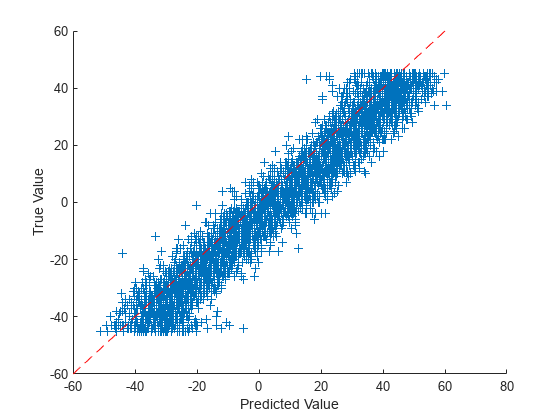
Visualize the predictions in a scatter plot. Plot the predicted values against the true values.
figure
scatter(YTest,anglesTest,"+")
xlabel("Predicted Value")
ylabel("True Value")

hold on
plot([-60 60], [-60 60],"r--")
See Also
trainnet | trainingOptions | dlnetwork