Create an Echometer Using Audio Measurements
This example shows how to create an echometer sonar using audio data acquisition and signal processing, which can measure distance by determining the time of flight of a sound pulse reflected off of a surface.
This example employs an approach for post synchronization of audio output and input data timestamps, which is required for applications where the input signal is in response to the output and/or when output/input timing correlation is relevant. Example applications include an acoustic characterization setup or stimulus-response experiments. The relative output/input lag is determined and corrected using correlation functions in Signal Processing Toolbox™.
Hardware Setup
Running this example requires:
Focusrite Scarlett 2i2 audio interface device, or another device / sound card with two output and two input audio channels
Audio interface device DirectSound drivers provided by the vendor, or using default Windows device drivers if available
One powered speaker and one microphone compatible with the audio interface device
Audio patch cables and connector adaptors
Typical DirectSound audio interface devices supported by Data Acquisition Toolbox™ do not support hardware synchronization between the output and input channels. Pairs of audio input or output channels are synchronized by the audio device, however the output and input channels can have a non-negligible relative start lag.
To synchronize the output and input data timestamps in post-processing, the following setup can be used:
Connect one of the output channels (output 1 or left channel of stereo plug) to one of the input channels (input 1 or left channel) to generate and acquire a synchronization signal in a loopback configuration.
The other output (output 2 or right channel) and input channel (input 2 or right channel) are used to output an excitation/stimulus signal, and respectively acquire a measurement/response signal.
Read data from both audio input channels, with one of the channels being used for reading the synchronization signal, and the other channel for reading the actual response signal.
With this setup, you read data from both audio input channels, and simultaneously write data to both audio output channels.
Echometer Sonar
As a demonstration of this approach, you can use an audio device, a powered speaker, and a microphone to put together an echometer sonar setup. A pulse echometer measures the distance to an object by emitting a short sound pulse, measuring the reflected pulse echo, and determining the time of flight by comparing the original output pulse signal with the measured input response signal.
The speaker and microphone are placed next to each other and oriented toward a wall off of which the sound pulse reflects, as in the diagram below.

Synthesize Pulse Signal
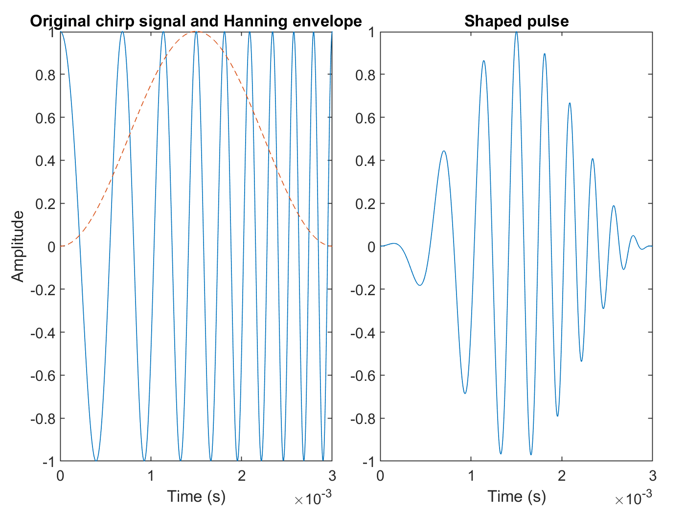
A pulse signal typically used for sonar applications is a short duration frequency sweep, or a chirp. Because the sharp amplitude edges at the beginning and end of a flat chirp signal can cause measurement artifacts, the pulse is attenuated/shaped by an envelope function. Options include Hanning, Gaussian, Kaiser, etc. Frequency range, pulse width or duration, pulse envelope/shape depend on the intended application. In this example the measurements are taken with a 3 ms duration pulse with a 1-5 kHz linear frequency chirp, and a Hanning window. The synthesized signal is shown in the figure below. The original chirp signal is shown on the left and the shaped pulse is shown on the right. The Hanning window is shown as a dotted line.
Make sure to use a signal frequency range that can be properly generated by the speaker, picked up by the microphone, and sampled by the audio interface device. The sampling rate used for the audio device measurements is 192 kHz.
% Pulse width (s)
T = 3E-3;

% Sampling rate (Hz)
Fs = 192E+3;

% Initial and final pulse frequency (Hz)
f0 = 1E+3;
f1 = 5E+3;

% Time vector
t = (0:1/Fs:T)';

% Pulse signal, chirp attenuated by an windowing function
yc = chirp(t,f0,t(end),f1);
w = hann(numel(t));
y = yc.*w;

% Plot the signal
figure
tileplot = tiledlayout(1,2);
tileplot.TileSpacing = 'compact';
tileplot.Padding = 'compact';

nexttile
plot(t,yc)
hold on
plot(t,w,'--')
xlabel("Time (s)")
ylabel("Amplitude")
title("Original chirp signal and Hanning envelope")

nexttile
plot(t,y)
xlabel("Time (s)")
title("Shaped pulse")
Data Acquisition
Use two separate DataAcquisition objects, one for the audio output channels and one for the audio input channels. Since there is no automatic synchronization possible between the audio input and output channel pairs even if a common DataAcquisition object is used for all channels, this approach allows for more control over the data acquisition operations.
do = daq("directsound");
addoutput(do,"Audio4","1","Audio");
addoutput(do,"Audio4","2","Audio");
do.Rate = Fs;

di = daq("directsound");
addinput(di,"Audio1","1","Audio");
addinput(di,"Audio1","2","Audio");
di.Rate = Fs;
Since the pulse duration is relatively short, pad the ending of the pulse signal with zero values (200 ms duration) to ensure that the pulse is generated correctly.
yout = [y; zeros(Fs*200E-3,1)];
Start the input first as a continuous background acquisition, then generate the same signal on both audio output channels. One of the channels is used as a synchronization signal.
start(di,"continuous")
write(do,[yout yout])
stop(di)
Read the acquired data into the workspace. By default, the read function returns a timetable.
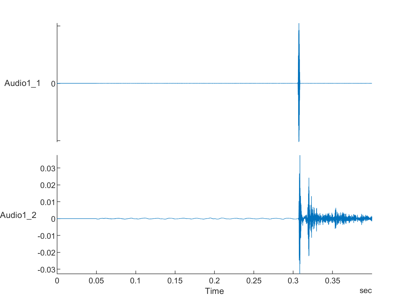
data = read(di,"all");Plot the acquired data. Signals Audio1_1 and Audio1_2 correspond to the audio input channels 1 and 2. Input channel 1 was used to record the synchronization signal generated by output channel 1 in a loopback configuration. Input channel 2 was used to record the actual response signal picked by the microphone. Two pulses are observed in the response signal, followed by other secondary echoes which depend on the room acoustics. Also notice the large relative start lag time between the input and output channels.
figure
stackedplot(data)
Synchronize Output and Input Data Timestamps
Find the lag and align the output and input signal timestamps by discarding the points before the detected synchronization signal.
lag = finddelay(y, data.Audio1_1);
t0 = lag/Fs
t0 = 0.3058
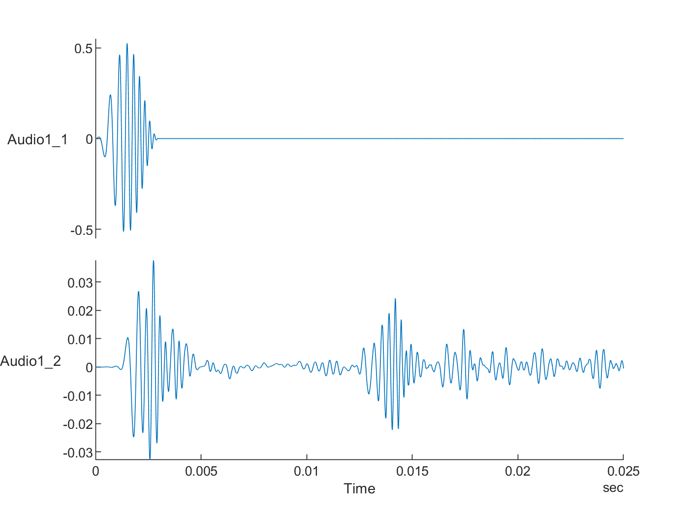
alignedData = data(lag+1:end,:);
alignedData.Time = alignedData.Time-alignedData.Time(1);

figure
s = stackedplot(alignedData);
xlim(seconds([0 0.025]))
s.AxesProperties(1).YLimits = [-0.55 0.55];
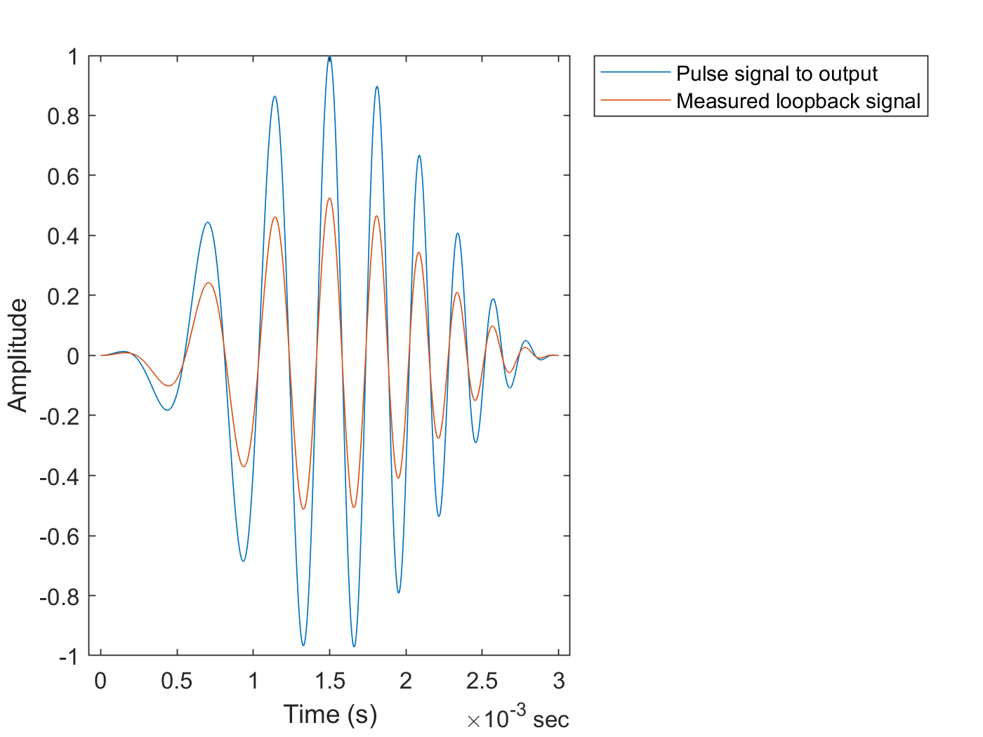
Visually validate the quality of the time alignment, by comparing the synthetic pulse data with the measured loopback signal.
figure
plot(seconds(t),y,alignedData.Time(1:numel(t)),alignedData.Audio1_1(1:numel(t)))
ylabel("Amplitude")
xlabel("Time (s)")
legend(["Pulse signal to output","Measured loopback signal"],"Location","bestoutside")
Determine Pulse Propagation Time and Distance
You can use the xcorr cross-correlation function to determine and visualize similarities between the original pulse signal and the measured response signal.
[xCorr,lags] = xcorr(alignedData.Audio1_2,y);

figure
plot(lags/Fs,xCorr)
xlabel('Lags (s)')
ylabel('Cross-correlation')
axis tight
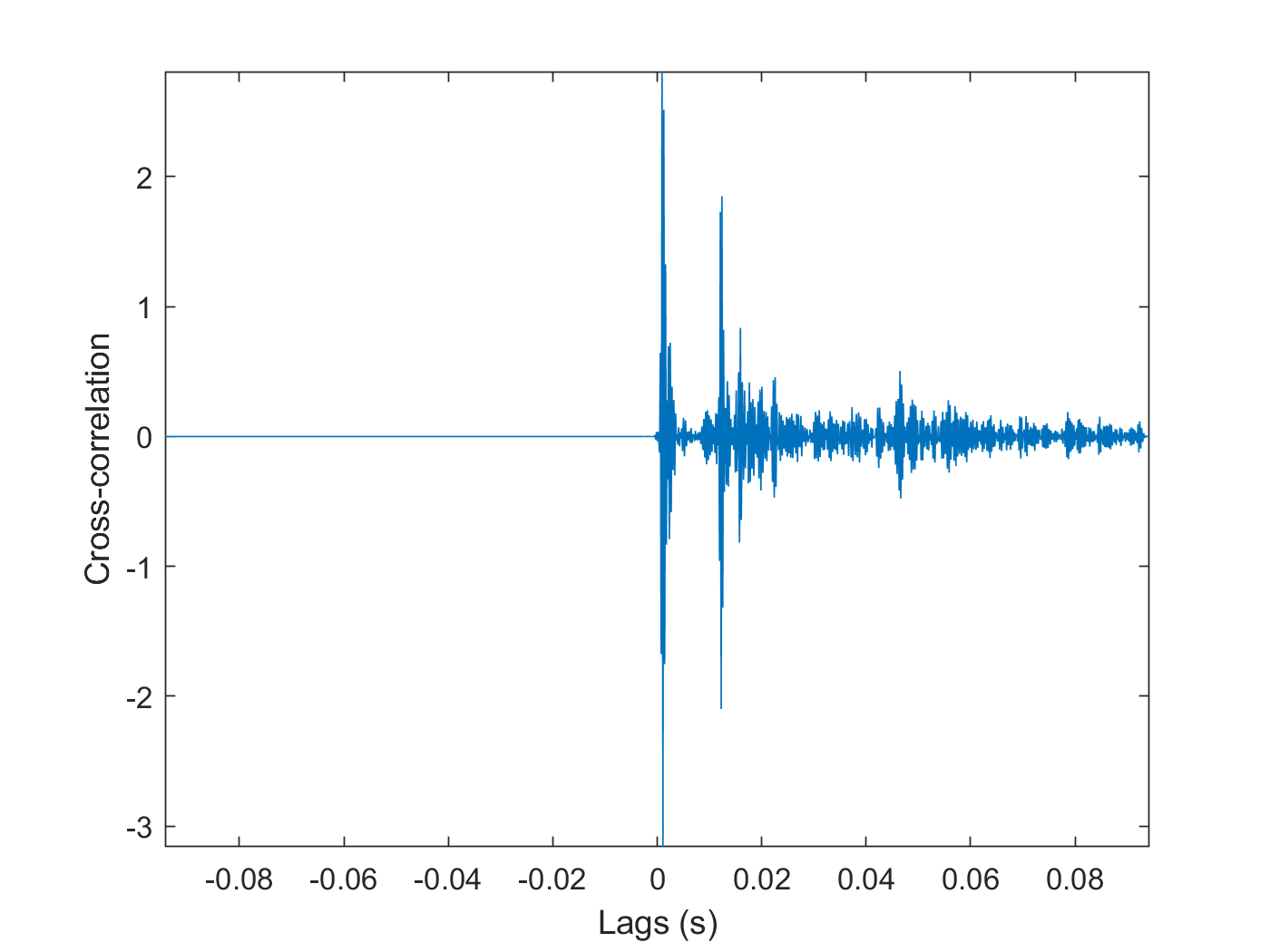
The cross-correlation plot indicates several similarities, with two larger peaks and other smaller peaks from reverberations.
Find timestamp and total propagation distance corresponding to the first two observed correlated pulses in the measured signal. The first observed pulse corresponds to the direct propagation path from the speaker to the microphone. The second observed pulse is the echo pulse reflected by the wall. The function finddelay returns the lag for which the normalized cross-correlation has the highest value, and in this case it corresponds to the first pulse in the response signal.
t1 = finddelay(y,alignedData.Audio1_2)/Fs
t1 = 0.0011
You can calculate the propagation time of the echo pulse as the starting timestamp of the second pulse in the response signal by using finddelay in the signal region after the first pulse.
t2 = t1 + T + finddelay(y,alignedData(timerange(seconds(t1+T),"inf"),:).Audio1_2)/Fst2 = 0.0122
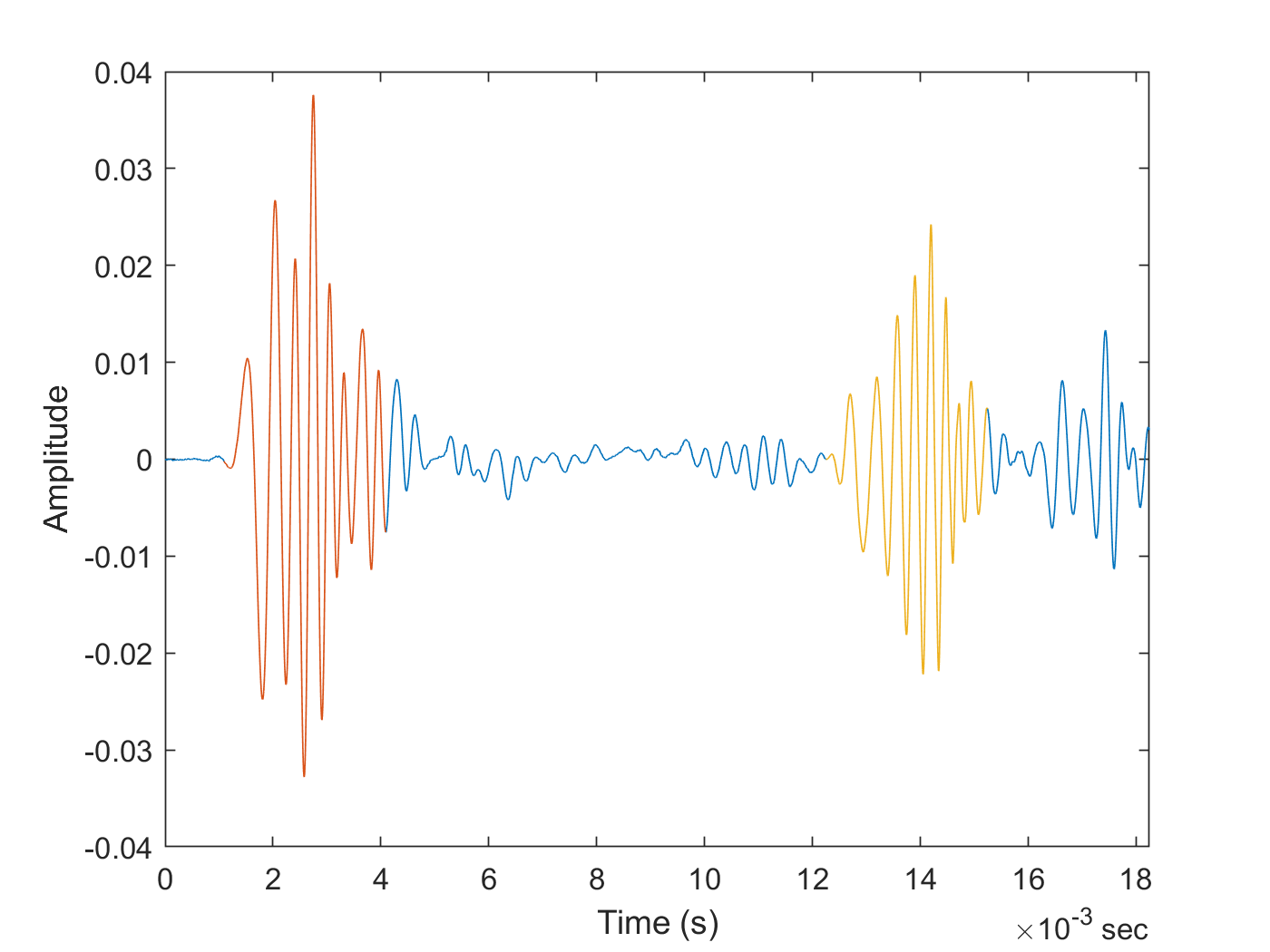
% Plot the response signal and highlight the first two detected pulses
figure
plot(alignedData.Time,alignedData.Audio1_2)
xlim(seconds([0 t2+2*T]))

hold on
firstPulse = alignedData(timerange(seconds(t1),seconds(t1+T)),:);
plot(firstPulse.Time,firstPulse.Audio1_2)

echoPulse = alignedData(timerange(seconds(t2),seconds(t2+T)),:);
plot(echoPulse.Time,echoPulse.Audio1_2)
ylabel("Amplitude")
xlabel("Time (s)")
% Calculate distance corresponding to echo pulse (m)
% Speed of sound in air at 20 deg. C (m/s)
v = 343.1;
d2 = t2*v/2
d2 = 2.1006
The distance (2.10 m) measured by the echometer sonar setup (half of the total path) is very close to the actual distance (2.06 m) between the speaker/microphone setup and the wall reflecting the echo pulse.