Evaluate a Surface Fit

This example shows how to work with a surface fit.

Load Data and Fit a Polynomial Surface

load franke;
surffit = fit([x,y],z,'poly23','normalize','on')

     Linear model Poly23:
     surffit(x,y) = p00 + p10*x + p01*y + p20*x^2 + p11*x*y + p02*y^2 + p21*x^2*y 
                    + p12*x*y^2 + p03*y^3
       where x is normalized by mean 1982 and std 868.6
       and where y is normalized by mean 0.4972 and std 0.2897
     Coefficients (with 95% confidence bounds):
       p00 =      0.4253  (0.3928, 0.4578)
       p10 =      -0.106  (-0.1322, -0.07974)
       p01 =     -0.4299  (-0.4775, -0.3822)
       p20 =     0.02104  (0.001457, 0.04062)
       p11 =     0.07153  (0.05409, 0.08898)
       p02 =    -0.03084  (-0.05039, -0.01129)
       p21 =     0.02091  (0.001372, 0.04044)
       p12 =     -0.0321  (-0.05164, -0.01255)
       p03 =      0.1216  (0.09929, 0.1439)

The output displays the fitted model equation, the fitted coefficients, and the confidence bounds for the fitted coefficients.

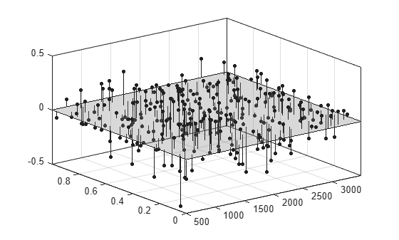
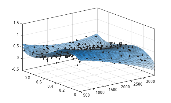
Plot the Fit, Data, Residuals, and Prediction Bounds

plot(surffit,[x,y],z)

Plot the residuals fit.

plot(surffit,[x,y],z,'Style','Residuals')

Plot prediction bounds on the fit.

plot(surffit,[x,y],z,'Style','predfunc')

Evaluate the Fit at a Specified Point

Evaluate the fit at a specific point by specifying a value for x and y , using this form: z = fittedmodel(x,y).

surffit(1000,0.5)

ans = 0.5673

Evaluate the Fit Values at Many Points

xi = [500;1000;1200];
yi = [0.7;0.6;0.5];
surffit(xi,yi)

ans = 3×1

    0.3771
    0.4064
    0.5331

Get prediction bounds on those values.

[ci, zi] = predint(surffit,[xi,yi])

ci = 3×2

    0.0713    0.6829
    0.1058    0.7069
    0.2333    0.8330

zi = 3×1

    0.3771
    0.4064
    0.5331

Get the Model Equation

Enter the fit name to display the model equation, fitted coefficients, and confidence bounds for the fitted coefficients.

surffit

     Linear model Poly23:
     surffit(x,y) = p00 + p10*x + p01*y + p20*x^2 + p11*x*y + p02*y^2 + p21*x^2*y 
                    + p12*x*y^2 + p03*y^3
       where x is normalized by mean 1982 and std 868.6
       and where y is normalized by mean 0.4972 and std 0.2897
     Coefficients (with 95% confidence bounds):
       p00 =      0.4253  (0.3928, 0.4578)
       p10 =      -0.106  (-0.1322, -0.07974)
       p01 =     -0.4299  (-0.4775, -0.3822)
       p20 =     0.02104  (0.001457, 0.04062)
       p11 =     0.07153  (0.05409, 0.08898)
       p02 =    -0.03084  (-0.05039, -0.01129)
       p21 =     0.02091  (0.001372, 0.04044)
       p12 =     -0.0321  (-0.05164, -0.01255)
       p03 =      0.1216  (0.09929, 0.1439)

To get only the model equation, use formula.

formula(surffit)

ans = 
'p00 + p10*x + p01*y + p20*x^2 + p11*x*y + p02*y^2 + p21*x^2*y + p12*x*y^2 + p03*y^3'

Get Coefficient Names and Values

Specify a coefficient by name.

p00 = surffit.p00

p00 = 0.4253

p03 = surffit.p03

p03 = 0.1216

Get all the coefficient names. Look at the fit equation (for example, f(x,y) = p00 + p10*x...) to see the model terms for each coefficient.

coeffnames(surffit)

ans = 9x1 cell
    {'p00'}
    {'p10'}
    {'p01'}
    {'p20'}
    {'p11'}
    {'p02'}
    {'p21'}
    {'p12'}
    {'p03'}

Get all the coefficient values.

coeffvalues(surffit)

ans = 1×9

    0.4253   -0.1060   -0.4299    0.0210    0.0715   -0.0308    0.0209   -0.0321    0.1216

Get Confidence Bounds on the Coefficients

Use confidence bounds on coefficients to help you evaluate and compare fits. The confidence bounds on the coefficients determine their accuracy. Bounds that are far apart indicate uncertainty. If the bounds cross zero for linear coefficients, this means you cannot be sure that these coefficients differ from zero. If some model terms have coefficients of zero, then they are not helping with the fit.

confint(surffit)

ans = 2×9

    0.3928   -0.1322   -0.4775    0.0015    0.0541   -0.0504    0.0014   -0.0516    0.0993
    0.4578   -0.0797   -0.3822    0.0406    0.0890   -0.0113    0.0404   -0.0126    0.1439

Find Methods

List every method that you can use with the fit.

methods(surffit)

Methods for class sfit:

argnames       category       coeffnames     coeffvalues    confint        dependnames    differentiate  feval          fitoptions     formula        indepnames     islinear       numargs        numcoeffs      plot           predint        probnames      probvalues     quad2d         setoptions     sfit           type           

Use the help command to find out how to use a fit method.

help sfit/quad2d

 QUAD2D  Numerically integrate a surface fit object.
    Q = QUAD2D(FO, A, B, C, D) approximates the integral of the surface fit
    object FO over the planar region A <= x <= B and C(x) <= y <= D(x). C and D
    may each be a scalar, a function handle or a curve fit (CFIT) object.
 
    [Q,ERRBND] = QUAD2D(...) also returns an approximate upper bound on the
    absolute error, ERRBND.
 
    [Q,ERRBND] = QUAD2D(FUN,A,B,C,D,PARAM1,VAL1,PARAM2,VAL2,...) performs
    the integration with specified values of optional parameters. 
 
    See QUAD2D for details of the upper bound and the optional parameters. 
      
    See also: QUAD2D, FIT, SFIT, CFIT.

×

Open Example

You have a modified version of this example. Do you want to open this example with your edits?

No, overwrite the modified version Yes