Analyze Dynamic Systems with Time Delays
You can use plotting commands such as stepplot and bodeplot analyze systems with time delays. The software makes no approximations when performing such analysis.
For example, consider the following control loop, where the plant is modeled as first-order plus dead time.
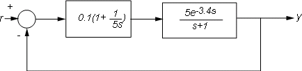
You can model the closed-loop system from r to y.
s = tf("s");
P = 5*exp(-3.4*s)/(s+1);
C = 0.1 * (1 + 1/(5*s));
T = feedback(P*C,1);
T is a state-space model with an internal delay. For more information about models with internal delays, see Closing Feedback Loops with Time Delays.
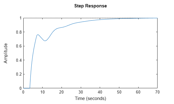
Plot the step response of T.
stepplot(T)
For more complicated interconnections, you can name the input and output signals of each block and use connect to automatically take care of the wiring. Suppose, for example, that you want to add a feedforward path to the control loop of the previous model.
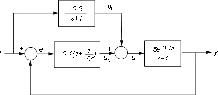
You can derive the corresponding closed-loop model Tff.
F = 0.3/(s+4);
P.InputName = "u";
P.OutputName = "y";
C.InputName = "e";
C.OutputName = "uc";
F.InputName = "r";
F.OutputName = "uf";
Sum1 = sumblk("e = r - y");
Sum2 = sumblk("u = uf + uc");
Tff = connect(P,C,F,Sum1,Sum2,"r","y");
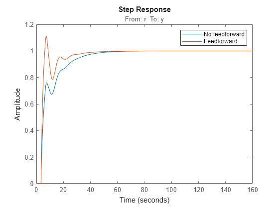
You can then compare its response with the feedback only design.
stepplot(T,Tff)
legend("No feedforward","Feedforward",Location="southeast")
Considerations When Analyzing Systems with Internal Delays
The time and frequency responses of delay systems can look odd and suspicious to those only familiar with delay-free LTI analysis. Time responses can behave chaotically, Bode plots can exhibit gain oscillations, and so on. These are not software or numerical quirks but real features of such systems. The following plots demonstrate some of these behaviors.
Gain Ripple
s = tf("s");
G = exp(-5*s)/(s+1);
T = feedback(G,.5);
bodemag(T)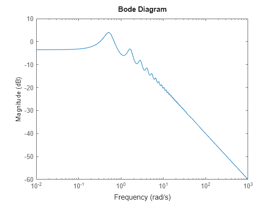
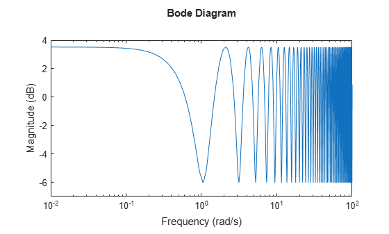
Gain Oscillations
G = 1 + 0.5 * exp(-3*s);
bodemag(G)
Jagged Step Response
G = exp(-s) * (0.8*s^2+s+2)/(s^2+s);
T = feedback(G,1);
stepplot(T)
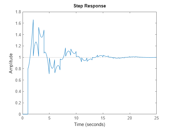
Here, the response includes echoes of the initial step function.
Chaotic Response
G = 1/(s+1) + exp(-4*s);
T = feedback(1,G);
stepplot(T,150)
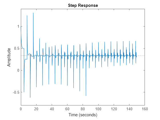
You can use Control System Toolbox™ tools to model and analyze these and other strange-appearing artifacts of internal delays.