SparseBalancedTruncation

R2026b

Sparse balanced truncation model order reduction object

Since R2023b

Description

The SparseBalancedTruncation object stores model order reduction (MOR) specifications for the balanced truncation of sparse linear time-invariant (LTI) models.

Creation

The reducespec function creates a sparse balanced truncation model order reduction object when you use this syntax.

R = reducespec(sys,"balanced")

Here, sys is a sparse LTI model (sparss, mechss). The workflow uses this object to set up MOR tasks and store results. For the full model order reduction workflow, see Task-Based Model Order Reduction Workflow.

Properties

Sigma — Hankel singular values

Read-only: [] (default) | vector

This property is read-only.

Hankel singular values, returned as a vector of size n-by-1. Here, n depends on the size of the rank of low-rank Gramian factors L_r and L_o. Additionally, n ≪ N, where N is the number of states of the original model.

In state coordinates that equalize the input-to-state and state-to-output energy transfers, the Hankel singular values (HSVs) measure the contribution of each state to the input/output behavior. Hankel singular values relate to model order as singular values relate to matrix rank. In particular, small HSVs indicate states that you can discard to simplify the model.

Energy — Normalized state energy

Read-only: [] (default) | vector

This property is read-only.

Normalized state energy in balanced coordinates, returned as a vector of size n-by-1. Here, n depends on the size of the rank of low-rank Gramian factors L_r and L_o. Additionally, n ≪ N, where N is the number of states of the original model.

These values measure the energy of each state relative to the state with maximum energy. The normalized state energy for the kth HSV is given by $${\left(\frac{{\sigma }_k}{{\sigma }_1}\right)}^2$$.

In balanced coordinates, the Hankel singular values σ are the eigenvalues of the equalized Gramians X_r = X_o. From

$$X_r={\displaystyle \underset{0}{\overset{\infty }{\int }}x(t)x{(t)}^T}dt$$

where $$x(t)=e^{tA}B$$ is the impulse response, you obtain the total state energy as follows:

$${\displaystyle \sum {\sigma }_i}=\text{tr}(X_r)={\displaystyle \underset{0}{\overset{\infty }{\int }}{\Vert x(t)\Vert }^{2}dt}$$

Hence, σ_k is the energy of kth principal state and $$\frac{{\sigma }_k}{{\sigma }_1}$$ is the normalized energy of kth principal state.

Error — Approximation error bound

Read-only: [] (default) | vector

This property is read-only.

Bound on the absolute approximation error, returned as a vector of size n-by-1. Here, n depends on the size of the rank of low-rank Gramian factors L_r and L_o. Additionally, n ≪ N, where N is the number of states of the original model.

Loss — Neglected fraction of state energy

Read-only: [] (default) | vector

Since R2024b

This property is read-only.

Neglected fraction of state energy, returned as a vector of size n-by-1. Here, n depends on the size of the rank of low-rank Gramian factors L_r and L_o. Additionally, n ≪ N, where N is the number of states of the original model.

For example, when you select an order r, the neglected fraction of total energy is given by:

$$\frac{{\displaystyle \sum _{i=r+1}^n{\sigma }_i}}{{\displaystyle \sum _{j=1}^n{\sigma }_j}}$$

Lr — Low-rank Cholesky factor of controllability Gramian

Read-only: [] (default) | matrix

This property is read-only.

Low-rank Cholesky factor of the controllability Gramian, returned as a matrix.

The controllability Gramian is approximately $$X_r\approx L_r{L}_r^T$$.

The computation of these low-rank approximations is based on [1] and [2].

Lo — Cholesky factor of observability Gramian

Read-only: [] (default) | matrix

This property is read-only.

Low-rank Cholesky factor of the observability Gramian, returned as a matrix.

The observability Gramian is approximately $$X_o\approx L_o{L}_o^T$$.

The computation of these low-rank approximations is based on [1] and [2].

Residuals — Residuals of Lyapunov equations

Read-only: [] (default) | 1-by-2 vector

This property is read-only.

Relative residuals of Lyapunov equations, returned as a 1-by-2 vector. This property helps you tell if the algorithm has converged.

InitialCondition — Initial condition subspace

Read-only: [] (default) | matrix

This property is read-only.

Initial condition subspace used for initial-condition-aware balanced truncation, returned as a matrix. The model order reduction algorithm preserves transient dynamics along the directions defined by the columns of this matrix.

When Options.InitialCondition is specified as a matrix, this property contains the same matrix.

When Options.InitialCondition is set to "auto", this property contains the automatically computed state directions. The algorithm selects these directions from the observability Gramian of the stable subsystem, using the energy threshold specified in the InitialConditionThreshold property.

If no initial-condition matching is used, this property is empty.

Options — Options for sparse balanced truncation

SparseBalancedTruncationOptions object

Options for balanced truncation of LTI models, specified as a SparseBalancedTruncationOptions object. Use dot notation to configure options for R. For example R.Options.Focus = [10 1e5].

For more information about available options, see SparseBalancedTruncationOptions.

Object Functions

process	Run model order reduction algorithm
view (balanced)	Plot state contributions when using balanced truncation method
getrom (balanced)	Obtain reduced-order models when using balanced truncation method

Examples

Sparse Balanced Truncation of Thermal Model

This example shows how to perform balanced truncation of a sparse state-space model obtained from linearizing a thermal model of heat distribution in a circular cylindrical rod.

Load the model data.

load cylindricalRod.mat
sys = sparss(A,B,C,D,E);
size(sys)

Sparse state-space model with 3 outputs, 1 inputs, and 7522 states.

The thermal model contains 7522 states.

Create a balanced truncation specification object for sys and run the algorithm.

R = reducespec(sys,"balanced");
R = process(R)

Initializing...
Running ADI with built-in shifts.........
Solved Lyapunov equations to desired accuracy.

R = 
  SparseBalancedTruncation with properties:

               Sigma: [36×1 double]
              Energy: [36×1 double]
               Error: [36×1 double]
                  Lr: [7522×36 double]
                  Lo: [7522×123 double]
           Residuals: [6.1259e-09 1.6131e-09]
    InitialCondition: []
             Options: [1×1 mor.SparseBalancedTruncationOptions]

Use the view command to visualize the state contributions as Hankel singular values.

view(R,"sigma")

Obtain the reduced-order model with maximum error of 1e-6. This results in a model with order 8.

rsys = getrom(R,MaxError=1e-6,Method="truncate");

Compare the singular value response of the models.

w = logspace(-7,-3,20);
fsys = frd(sys,w);
sigma(fsys,fsys-rsys,'r--')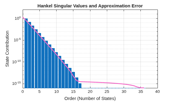

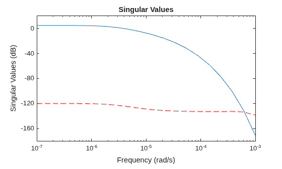
The reduced-order model is a good match for the full-order model.

Sparse Balanced Truncation of Thermal Model with Initial Condition

This example shows how to simplify a large-scale thermal model in a way that preserves both its input/output response and its response to specific initial conditions.

Load the model data.

load cylindricalRod.mat
rng default
n = size(A,1);
B = sparse(n,1);
B(randi(n,500,1)) = 1;
sys = sparss(A,B,C,D,E);
size(sys)

Sparse state-space model with 3 outputs, 1 inputs, and 7522 states.

The thermal model contains 7522 states.

Standard Balanced Truncation

First perform standard model reduction with balanced truncation. This method lets you approximate the input/output response to the desired fidelity.

R = reducespec(sys, "balanced");
R = process(R);

Initializing...
Running ADI with built-in shifts.........
Solved Lyapunov equations to desired accuracy.

Obtain the reduced-order model with maximum error of 1e-4. This results in a model with order 17.

[rsys, info] = getrom(R,MaxError=1e-4,Method="truncate");

Prepare data for simulation.

T = 1e-2;
N = 1000;
t = linspace(0,T,N)';
u = sin(5*2*pi/T*t);

Simulate both the original and reduced models with the input u.

y = lsim(sys,u,t);
yr = lsim(rsys,u,t);
plot(t,y,'b',t,yr,'r--')
legend({'y', '', '', 'yr', '', ''})

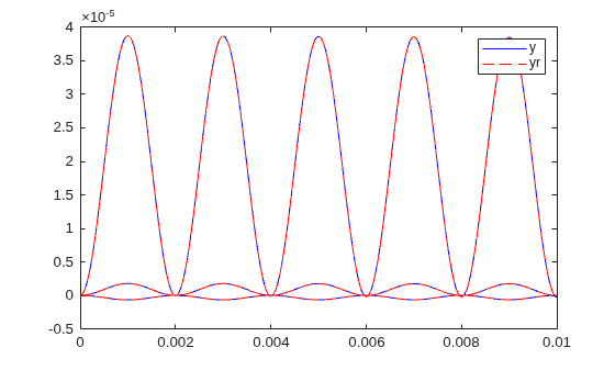
The plot shows that the reduced model captures the dynamics very well.

Now repeat the comparison with a nonzero initial condition x0. Scale x0 so that the input response and initial condition response have similar magnitudes.

x0 = 6e-5*randn(order(sys),1);

The reduced initial condition x0r corresponding to x0 is given by

x0r = info.PX'*x0;

Simulate and compare the original and reduced models responses in time domain.

y = lsim(sys,u,t,x0);
yr = lsim(rsys,u,t,x0r);
plot(t,y,'b',t,yr,'r--')
legend({'y', '', '', 'yr', '', ''})

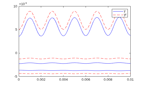
The plot shows that there is a visible gap between the full-order and reduced-order responses. To preserve the contribution of the initial condition x0, you must use augmented balanced truncation.

Balanced Truncation with Initial Condition

Generate a basis for the space of initial conditions automatically by setting options to "auto". This setting enables augmented balanced truncation where initial condition is taken into account during model reduction process.

R_IC = reducespec(sys,"balanced");
R_IC.Options.InitialCondition = 'auto';
R_IC = process(R_IC);

Initializing...
Running ADI with built-in shifts.........
Solved Lyapunov equations to desired accuracy.
Initializing...
Running ADI with built-in shifts.........
Solved Lyapunov equations to desired accuracy.

Obtain the reduced-order model with maximum error of 1e-4. This results in a model with order 36.

[rsys_IC, info_IC] = getrom(R_IC,MaxError=1e-4,Method="truncate");

Obtain Initial condition x0r and simulate the response to both u and the initial condition.

x0r_IC = info_IC.PX'*x0;
y = lsim(sys,u,t,x0);
yr_IC = lsim(rsys_IC,u,t,x0r_IC);
plot(t,y,'b',t,yr_IC,'r--')
legend({'y', '', '', 'yr_{IC}', '', ''})

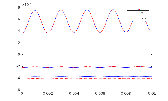
The augmented model improves the combined response, but one output channel still deviates. You can improve accuracy by using a larger initial-condition subspace.

Increase Initial-Condition Basis Size

R_IC.Options.InitialConditionThreshold = 1e-6;
R_IC = process(R_IC);

Initializing...
Running ADI with built-in shifts.........
Solved Lyapunov equations to desired accuracy.
Initializing...
Running ADI with built-in shifts.........
Solved Lyapunov equations to desired accuracy.

Obtain the reduced-order model with maximum error of 1e-4. This results in a model with order 53.

[rsys_IC, info_IC] = getrom(R_IC,MaxError=1e-4,Method="truncate");

Obtain Initial condition x0r and simulate the response to both u and the initial condition.

x0r_IC = info_IC.PX'*x0;
y = lsim(sys,u,t,x0);
yr_IC = lsim(rsys_IC,u,t,x0r_IC);
plot(t,y,'b',t,yr_IC,'r--')
legend({'y', '', '', 'yr_{IC}', '', ''})

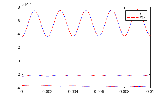
Now both the input response and initial-condition response closely match the full model.

Testing Multiple Initial Conditions

Test the reduced model with 10 random initial conditions.

err = zeros(10,1);
for i = 1:10
    x0 = randn(order(sys),1);
    x0r_IC = info_IC.PX'*x0;
    y = lsim(sys,u,t,x0);
    yr_IC = lsim(rsys_IC,u,t,x0r_IC);
    err(i) = norm(y(:) - yr_IC(:))/norm(y(:));
end
err

err = 10×1

    0.0008
    0.0007
    0.0010
    0.0005
    0.0008
    0.0015
    0.0008
    0.0024
    0.0005
    0.0003

All relative trajectory errors are below 0.3%, demonstrating excellent fidelity for a wide range of initial conditions.

Add Rayleigh Damping to Enforce Stability for Sparse Balanced Truncation

This example shows how to perform balanced truncation of an undamped second-order sparse model of a cantilever beam. Sparse balanced truncation is only supported for stable systems, but the algorithm allows you to implicitly add Rayleigh damping and enforce stability to perform model order reduction.

Load the beam model.

load linBeam.mat
size(sys)

Sparse second-order model with 1 outputs, 1 inputs, and 3303 degrees of freedom.

Plot the Bode response.

fsys = frd(sys,w);
bode(fsys)

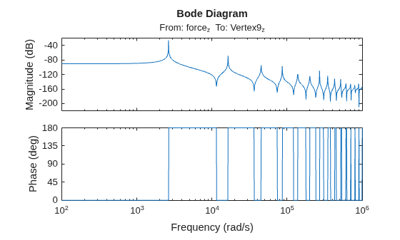
The response shows that the model is undamped and has a dominant mode at 2639 rad/s.

Create a model order reduction task.

R = reducespec(sys,"balanced");

Add the Rayleigh damping. Specify the natural frequency at 2700 rad/s near the dominant mode and the damping as 0.01.

R.Options.Rayleigh = [2700,0.01];

Analyze the model and compute the derived information.

R = process(R);

Initializing...
Running ADI with built-in shifts........................................
.............................
Running ADI with adaptive shifts........
Solved Lyapunov equations to desired accuracy.

Obtain a reduced-order model with order 20.

rsys = getrom(R,Order=20,Method="truncate");
bode(fsys,rsys,"r--",w)
legend("Original sparse model","Reduced model")

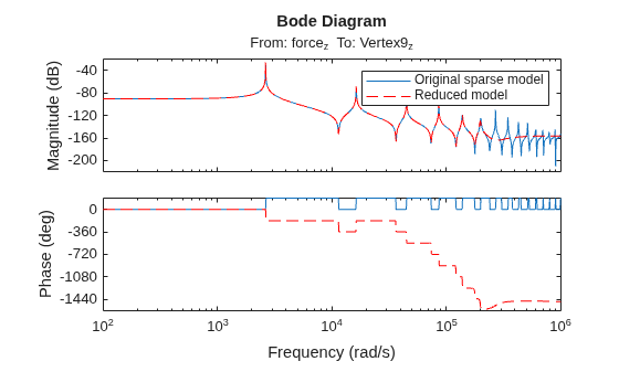
The reduced-order model is a good match for the sparse model.

Algorithms

The sparse balanced truncation algorithm performs these steps to reduce the input model G to the desired order k.

1. Find the low-rank approximations L_r and L_o of the Gramian factors. This is based on the low-rank alternating directions implicit (LRADI) algorithm, which is an iterative method for solving the Lyapunov equations. For more details, see [1] and [2].

2. Compute the HSVs σ_j based on the approximate controllability and observability Gramians.

3. Obtain the reduced order model using the balanced model truncation with absolute error control [3] (see the Algorithms section of BalancedTruncation).

References

[1] Benner, Peter, Jing-Rebecca Li, and Thilo Penzl. “Numerical Solution of Large-Scale Lyapunov Equations, Riccati Equations, and Linear-Quadratic Optimal Control Problems.” Numerical Linear Algebra with Applications 15, no. 9 (November 2008): 755–77. https://doi.org/10.1002/nla.622.

[2] Benner, Peter, Martin Köhler, and Jens Saak. “Matrix Equations, Sparse Solvers: M-M.E.S.S.-2.0.1—Philosophy, Features, and Application for (Parametric) Model Order Reduction.” In Model Reduction of Complex Dynamical Systems, edited by Peter Benner, Tobias Breiten, Heike Faßbender, Michael Hinze, Tatjana Stykel, and Ralf Zimmermann, 171:369–92. Cham: Springer International Publishing, 2021. https://doi.org/10.1007/978-3-030-72983-7_18.

[3] Varga, A. “Balancing Free Square-Root Algorithm for Computing Singular Perturbation Approximations.” In [1991] Proceedings of the 30th IEEE Conference on Decision and Control, 1062–65. Brighton, UK: IEEE, 1991. https://doi.org/10.1109/CDC.1991.261486.

Version History

Introduced in R2023b

R2024b: Select model order using new criteria based on total neglected state energy

You can now select model order based on the fraction of total energy you want to neglect. The BalancedTruncation and SparseBalancedTruncation objects now contain a new property Loss to store the energy loss as a fraction of total energy, and getrom provides a new name-value argument MaxLoss to pick the reduced order based on maximum energy loss as a fraction of total energy. For example, to obtain a reduced model which neglects 1% of the total energy, you can specify rsys = getrom(R,MaxLoss=0.01).