Adaptive Equalization with Filtering and Fading Channel

This model shows the behavior of the selected adaptive equalizer in a communication link that has a fading channel. The transmitter and receiver have root raised cosine pulse shaped filtering. A subsystem block enables you to select between linear or decision feedback equalizers that use the least mean square (LMS) or recursive least square (RLS) adaptive algorithm.

Model Structure

• The transmitter generates 16QAM random signal data that includes a training sequence and applies root raised cosine pulse shaped filtering.

• Channel impairments include multipath fading, Doppler shift, carrier frequency offset, variable integer delay, free space path loss, and AWGN.

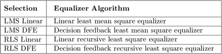
• The receiver applies root raised cosine pulse shaped filtering, adjusts the gain, includes equalizer mode control to enable training and enables you to select the equalizer algorithm from these choices.

• Scopes help you understand how the different equalizers and adaptive algorithms behave.

Explore Example Model

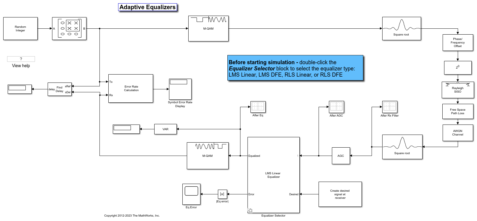
Experimenting with the model

This model provides several ways for you to change settings and observe the results. The model uses callback functions to configure some block and subsystem parameters. For more information, see Model Callbacks (Simulink). The InitFcn callback function, found in Modeling>Model Settings>Model Properties>Callbacks, calls the cm_ex_adaptive_eq_with_fading_init helper function to initialize the model. This helper function enables you to vary settings in the model, including:

• System parameters, such as SNR.

• Pulse shaping filter parameters, such as rolloff and filter length.

• Path loss value.

• Channel conditions: Rayleigh or Rician fading, channel path gains, channel path delays, and Doppler shift.

• Equalizer choice and configuration, as used by the Equalizer Selector subsystem.

Model Considerations

This non-standards-based communication link is representative of a modern communications system.

• The optimal equalizer configuration depends on the channel conditions. The initialization helper function sets the Doppler shift and multipath fading channel parameters that highlight the capabilities of different equalizers.

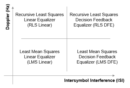
• The decision feedback equalizer structure performs better than the linear equalizer structure for higher intersymbol interference.

• The RLS algorithm performs better than the LMS algorithm for higher Doppler frequencies.

• The LMS algorithm executes quickly, converges slowly, and its complexity grows linearly with the number of weights.

• The RLS algorithm converges quickly, its complexity grows approximately as the square of the number of weights. It can be unstable when the number of weights is large.

• The channels exercised for different equalizers have the following characteristics.

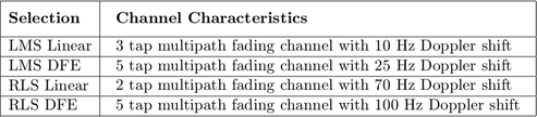
• Initial settings for other channel impairments are the same for all equalizers. Carrier frequency offset value is set to 50 Hz. Free space path loss is set to 60 dB. Variable integer delay is set to 2 samples, which requires the equalizers to perform some timing recovery.

Deep channel fades and path loss can cause the equalizer input signal level to be much less than the desired output signal level and result in unacceptably long equalizer convergence time. The AGC block adjusts the magnitude of received signal to reduce the equalizer convergence time. You must adjust the optimal gain output power level based on the modulation scheme selected. For 16QAM, a desired output power of 10 W is used.

Training of the equalizer is performed at the beginning of the simulation.

Running the Simulation

Running the simulation computes symbol error statistics and produces these figures:

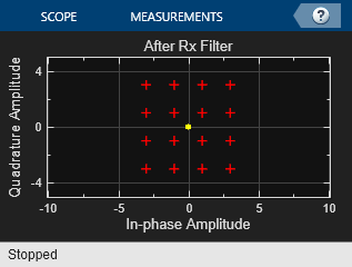
• A constellation diagram of the signal after the receive filter.

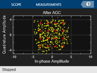
• A constellation diagram of the signal after adjusting gain.

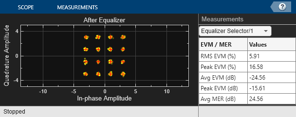
• A constellation diagram of the signal after equalization with signal quality measurements shown.

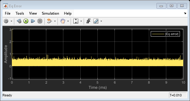
• An equalizer error plot.

For the plots shown here, the equalizer algorithm selected is RLS Linear. Monitoring these figures, you can see that the received signal quality fluctuates as simulation time progresses.

The After Rx Filter and After AGC constellation plots show the signal before equalization. After AGC shows the impact of the channel conditions on the transmitted signal. The After Eq plot shows the signal after equalization. The signal plotted in the constellation diagram after equalization shows the variation in signal quality based on the effectiveness of the equalization process. Throughout the simulation, the signal constellations plotted before equalization deviate noticeably from a 16QAM signal constellation. The After Eq constellation improves or degrades as the equalizer error signal varies. The Eq error plotted in the Eq Error plot, indicates poor equalization at the start of the simulation. The error degrades at first then improves as the equalizer converges.

Further Exploration

Double-click the Equalizer Selector subsystem and select a different equalizer. Run the simulation to see the performance of the various equalizer options. You can use the signal logger to compare the results from this experimentation. In the model window, right-click on signal wires and select Log Selected Signals. If you have enabled signal logging, after the simulation run finishes, open the Simulation Data Inspector to view the logged signals.

At the MATLAB® command prompt, enter edit cm_ex_adaptive_eq_with_fading_init.m to open the initialization file, then modify a parameter and rerun the simulation. For example, adjust the channel characteristics (params.maxDoppler, params.pathDelays, and params.pathGains). The RLS adaptive algorithm performs better than the LMS adaptive algorithm as the maximum Doppler is increased.