Automated Design of Audio Filters for Room Equalization

This example combines Optimization Toolbox™ and Audio Toolbox™ to develop an algorithm that automatically tunes a set of filter parameters.

There are many audio applications where it is desirable to compute parametric equalizer parameters to fit an arbitrary frequency response. For instance, one could fit a filter response to a measured impulse response (IR) to obtain a lower-order implementation of the same filter. Alternatively, one can apply correction to a measured loudspeaker response (anechoic or in-room) to smooth out any imperfections and create a perceptually flat frequency response. The latter is demonstrated here by designing an algorithm that automatically tunes the parameters of N parametric equalizers such that when the resulting EQ is applied to the speaker, the frequency response is perceived as flat in the room.

This example goes over the following steps:

• Measure the in-room response of a loudspeaker using the Impulse Response Measurer

• Compute a fractional-octave smoothed response

• Take into account the microphone calibration data

• Compute a target response that is perceptually optimal for the given loudspeaker system and room configuration

• Optimize a set of filter parameters that modifies the response to better fit the target

• Produce an audio filter or audio files to evaluate the results using headphones or listening room

In-Room Measurement

The first step is to obtain measurements for the system that needs to be improved.

Set up a full duplex sound interface so that it can both play on the loudspeaker, and record with a calibration microphone (such as a Behringer ECM8000 connected to a sound interface capable of supplying phantom power). Place the microphone on a stand so that you can move it into the listening position(s). You can start with the microphone centered in the listener's position, but measuring at several positions will help reduce the chances of overcorrecting for issues like a high frequency dip in the response that could only be present in a region smaller than a listener's head.

Start the Impulse Response Measurer app by entering impulseResponseMeasurer at the command prompt. You can also click the app icon on the Apps tab of the MATLAB® Toolstrip.

Verify that the correct audio device is selected. Change the sample rate if desired (this example uses 96 kHz). Set the player and recorder channels to the loudspeaker and microphone, respectively.

Select the Swept Sine method. Set the number of runs to average several measurement together. This example uses five. Set the duration per run to have time for a long enough swept sine and a period of silence that is long enough for the reverberation to completely die off, which can be several seconds in a typical room.

In the advanced settings, set a pause between runs that allows time to move the microphone around the initial "center" position. You must keep silent during the "silence" part of the measurement, but you can move the microphone and make noise during this pause. The start frequency should be set below the range of the loudspeaker (10 Hz might be a good starting point). The stop frequency can be set to half the sampling rate, unless measuring a subwoofer with limited high-frequency range. Set the sweep duration to a few seconds, and make sure there is enough duration left for silence at the end.

You may test levels with the level meter or try a first capture with 1 short run. Set playback level loud enough to hide any background noise in the room and set the microphone level so that it is high but does not overload/clip.

Now you can capture and save export the data to a MAT file. The rest of this example uses a file provided here.

Import the Measurement

Import the last measurement that was exported by the application (by addressing with end). The data used here is in a similar (but compatible) format.

load('measured_ir_data.mat','measurementData');
Fs = measurementData.SampleRate(end);
ir = measurementData.ImpulseResponse(end).Amplitude;
frequency = measurementData.MagnitudeResponse(end).Frequency;
if isfield(measurementData.MagnitudeResponse,'PowerDb')
    magnitudeDB = measurementData.MagnitudeResponse(end).PowerDb;
else % Version R2022b of IRM has renamed this field to Magnitude (dB)
    magnitudeDB = measurementData.MagnitudeResponse(end).MagnitudeDB;
end

Using a helper function provided here, smooth the response by 1/24-octave sections. Since powerDB is a measurement, add extra smoothing (last argument set to true).

fullRange = [10,Fs/2]; % Full audio range (for the plots)
[powerFR,cfFR] = octaveAverage(frequency,db2mag(magnitudeDB),24,fullRange,true);
pdbFR = 20*log10(powerFR);

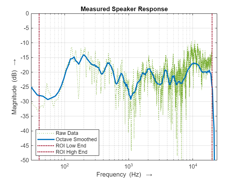
Plot the measurement and the smoothed response.

semilogx(frequency,magnitudeDB,':',Color="#77AC30")
hold on
plot(cfFR,pdbFR,'b',LineWidth=2,Color="#0072BD")
title('Measured Speaker Response')
legend('Raw Data','Octave Smoothed',Location='southwest')
xlabel('Frequency (Hz) \rightarrow')
ylabel('Magnitude (dB) \rightarrow')
yrange = [-50 0];
axis([30 22e3 yrange])
hold off
grid on

Microphone Calibration

If there is calibration data available for the microphone, subtract it from the measurement.

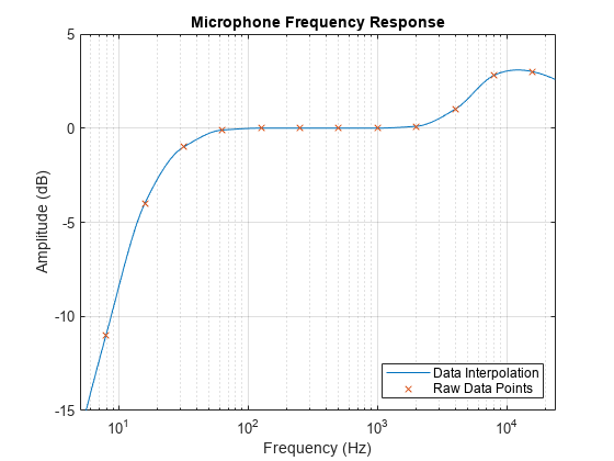
In this case, generic calibration data for the Behringer ECM8000 microphone is used. Calling the helper function with no output arguments plots the microphone frequency response.

getMicCalibration()

Subtract the microphone calibration data from the measured response, using the same frequency values.

micGainDB = getMicCalibration(cfFR);
pdbFRmic = pdbFR - micGainDB;

Determine a "range of interest" (ROI) for the optimization based on the measurement above and the manufacturer specifications for our loudspeaker. The bookshelf speaker measured above has a range of 60 Hz to 22 kHz according to the manufacturer. Set the ROI to a range of 40 Hz to 20 kHz to slightly increase the low end and to take into account the steep decline above 20 kHz.

ROI = [40 20e3]; % specify the region of interest for the optimization

Plot the corrected response and the ROI region.

semilogx(frequency,magnitudeDB,':',Color="#77AC30")
hold on
plot(cfFR,pdbFRmic,Color="#0072BD",LineWidth=2)
plot([ROI(1) ROI(1)],yrange,':',Color="#A2142F",LineWidth=1.5);
plot([ROI(2) ROI(2)],yrange,':',Color="#A2142F",LineWidth=1.5);
title('Measured Speaker Response')
legend('Raw Data','Octave Smoothed',...
       'ROI Low End','ROI High End',Location='southwest')
xlabel('Frequency (Hz) \rightarrow')
ylabel('Magnitude (dB) \rightarrow')
axis([30 24e3 -50 0])
hold off
grid on

Compute a Target Response

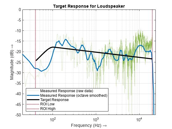
The next step is to determine a suitable target response for the system in the ROI. The main goal is to provide a response that is perceived as "flat", and potentially extend the low frequencies (within reasonable limits).

It is important to consider whether the response being optimized is a loudspeaker measurement in an anechoic chamber, or a loudspeaker in a room measured from a listening position. In the former case, the target could be a constant level (with a roll off outside of the loudspeaker's range). In the later case, which is the case for this example, the response at the listening position also depends on the room. The loudspeaker is perceived as "flat" if it exhibits a constant slope down. The degree of that slope depends on factors such as the distance of the listener. The perceived quality also depends on the low frequency cutoff point (approximately -10 dB), so the target curve can be used to extend the low frequencies if the boost remains moderate. Keep in mind that loudspeaker distortion increases in the lower frequencies, and the overall limits of the amplifier and loudspeaker should not be exceeded.

To compute a target response, fit a straight line (in the log-frequency domain) onto the frequency response (in dB) for a subset of the ROI. Add a roll off to the lower frequencies.

% Compute the octave average (only for the region of interest)
[power,cf] = octaveAverage(frequency,db2mag(magnitudeDB),24,ROI,true);
pdb = 20*log10(power) - getMicCalibration(cf);

% Set the range of the linear fit
lfCutOff = 2.5*ROI(1); % lowest frequency to linearize
hfMaxFit = 0.6*ROI(2); % max frequency to fit for

% Fit a straight line in the log-frequency domain
linIdx = cf>=lfCutOff & cf<=hfMaxFit;
if license('test','statistics_toolbox')
    pfit = robustfit(log(cf(linIdx)),pdb(linIdx));
else % if this toolbox is not available, use a simple linear regression
    pfit = [ones(nnz(linIdx),1) log(cf(linIdx))] \ pdb(linIdx);
end
targetResp = pfit(1)+pfit(2)*log(cf);

% Roll off the low frequencies, starting slightly above the linear range above
lfcutoff = 1.05*lfCutOff;
idx = cf<lfcutoff;
targetResp(idx) = targetResp(idx) - min(30,ROI(1)/2)*((lfcutoff-cf(idx))/lfcutoff).^2;

% Plot the target response
semilogx(frequency,magnitudeDB,':',Color="#77AC30");
hold on
axis([20 24e3 yrange]);
plot(cfFR,pdbFRmic,Color="#0072BD",LineWidth=2)
plot(cf,targetResp,Color="#000000",LineWidth=2.5);
plot([ROI(1) ROI(1)],yrange,':',Color="#A2142F",LineWidth=1.5);
plot([ROI(2) ROI(2)],yrange,':',Color="#A2142F",LineWidth=1.5);
title('Target Response for Loudspeaker');
legend('Measured Response (raw data)','Measured Response (octave smoothed)',...
       'Target Response','ROI Low','ROI High',Location='southwest')
xlabel('Frequency (Hz) \rightarrow')
ylabel('Magnitude (dB) \rightarrow')
grid on
hold off

The target response (in black) has a slight downward tilt and a roll off for the low frequencies that allows for some boost (10 to 12 dB).

Parametric Filter Overview

The variables being tuned by the optimization algorithm are typical audio parametric EQ parameters: Center Frequency, Filter Bandwidth, and Peak Gain.

Use the response to produce settings for a 12-band parametric filter (10 peak filters and 2 shelf filters).

Use the designParamEQ function from Audio Toolbox to design the filter. Use the lsqnonlin (Optimization Toolbox) function to perform the fit by tuning the parameters of the EQ bands until the speaker response is as flat as possible.

Before configuring the optimization algorithm, you can look at what a manual filter design looks like for 2 filters. Use the following controls to manually tune the filter parameters and observe the output response using filterAnalyzer. This allow us to visualize the parameters that the optimization algorithm automatically tunes.

gain = [4, ...
      -6.6]; 
  
centerFreq = [3520, ...
              7230]; 
          
bandwidth = [1920, ...
              4110];

Next, generate the filter coefficients using the specified parameters by calling designParamEQ:

[B,A] = designParamEQ(2,gain,(centerFreq/(Fs/2)),(bandwidth/(Fs/2)),Orientation='row');

Visualize the filter design.

filterAnalyzer(B,A,SampleRates=Fs)

Parametric Filter Optimization

To produce the optimized parametric filters, call a helper function that sets starting values and limits for every filter parameter, then calls lsqnonlin. The optimizer uses the eqObjectiveFct function that computes the response of the given EQ and compares it to the desired response. The lsqnonlin optimizer attempts to minimize that error on every iteration.

% Run the optimization with a selected number of filters
numFilters = 10+2; % 10 peak filters, one low shelf, and one high shelf
[EQ,outputResp] = eqOptimizer(numFilters,frequency,pdb,targetResp,ROI,Fs);

                                            Norm of      First-order 
 Iteration  Func-count      Resnorm            step       optimality
     0         37          0.162731                            0.425
     1         74         0.0545925              10            0.524      
     2        111         0.0290028              20            0.107      
     3        148         0.0279642         27.7143            0.223      
     4        185         0.0190037         6.92858            0.186      
     5        222         0.0154974        0.358522            0.173      
     6        259         0.0128502         13.8572            0.115      
     7        296         0.0100923         3.46429           0.0784      
     8        333         0.0100923         6.92858           0.0784      
     9        370        0.00950391         1.73215           0.0954      
    10        407         0.0082267         3.46429          0.00596      
    11        444          0.007321         6.92858           0.0923      
    12        481        0.00647468         13.8572           0.0382      
    13        518        0.00601745         27.7143           0.0407      
    14        555        0.00601745         27.7143           0.0407      
    15        592        0.00548673         6.92858           0.0454      
    16        629        0.00548673          14.993           0.0454      
    17        666        0.00496145         3.46429           0.0117      
    18        703         0.0044269         6.92858          0.00467      
    19        740         0.0044269         8.60961          0.00467      
    20        777        0.00405319          2.1524            0.022      
    21        814        0.00360236          4.3048          0.00209      
    22        851        0.00360236         7.15549          0.00209      
    23        888         0.0034787         1.78887           0.0176      
    24        925        0.00326625         2.29703           0.0188      
    25        962        0.00318511         1.50731           0.0188      
    26        999        0.00317997         1.78755          0.00471      
    27       1036        0.00317785        0.894889          0.00554      
    28       1073        0.00317591         0.63816          0.00235      
    29       1110        0.00317591         3.57775          0.00235      
    30       1147        0.00317558        0.894437          0.00106      
    31       1184        0.00317492        0.421078          0.00225      
    32       1221        0.00317459        0.816728            0.005      
    33       1258        0.00317438        0.894437          0.00287      
    34       1295        0.00317415        0.223609          0.00386      
    35       1332        0.00317407        0.223609          0.00138      
    36       1369          0.003174        0.447218         0.000363      
    37       1406        0.00317395        0.239862         0.000148      
    38       1443        0.00317394        0.447218          9.4e-05      
    39       1480        0.00317393        0.114499         5.44e-05      

Optimization stopped because the relative sum of squares (r) is changing
by less than options.FunctionTolerance = 1.000000e-08.

Results

Examine the results. Start by computing the filter frequency response over a larger frequency range.

freqzResp = eqFreqz(EQ,frequency,Fs);
pFR = octaveAverage(frequency,abs(freqzResp),24,fullRange,false);
filtRespFR = 20*log10(pFR);
outputRespFR = pdbFRmic + filtRespFR;

Plot the system response.

% Plot the system response
semilogx(frequency,magnitudeDB,':',Color="#77AC30");
hold on
axis([20 24e3 yrange]);
plot(cfFR,pdbFRmic,Color="#0072BD",LineWidth=2)
plot(cf,targetResp,Color="#000000",LineWidth=2.5);
plot([ROI(1) ROI(1)],yrange,':',Color="#A2142F",LineWidth=1.5);
plot([ROI(2) ROI(2)],yrange,':',Color="#A2142F",LineWidth=1.5);
plot(cfFR,outputRespFR,Color="#D95319",LineWidth=2);
title('Measured Speaker Response with and without EQ');
legend('Measured Response (raw data)',...
       'Measured Response (octave smoothed)',...
       'Target Response','ROI Low','ROI High',...
       'Corrected Response',Location='southwest')
xlabel('Frequency (Hz) \rightarrow')
ylabel('Magnitude (dB) \rightarrow')
grid on
hold off

Also plot error relative to target, but invert the error curves to make it easier to compare them with the optimized EQ.

% Plot error relative to target
errorOld = targetResp - pdb;
errorNew = targetResp - outputResp;
semilogx(cf([1,end]),[0,0],Color="#000000",LineWidth=2);
hold on;
plot(cf,errorOld,Color="#0072BD",LineWidth=2);
plot(cf,errorNew,Color="#77AC30",LineWidth=2);
plot(cfFR,filtRespFR,Color="#D95319",LineWidth=1.5);
hold off; grid on;
axis([20 24e3 -15 15])
title('Error Relative to Target');
xlabel('Frequency (Hz) \rightarrow');
ylabel('Magnitude (dB) \rightarrow');
legend('Target','Original Error (inverted)',...
       'Corrected Error (inverted)',...
       'Optimized EQ',Location='southwest');

Sort peak filters by center frequency and convert to table format.

EQpk = EQ(1:end-2,:);
[~,idx] = sort(EQpk(:,3));
EQ(1:end-2,:) = EQpk(idx,:);

% Create a table with all the EQ settings
filterType =  [repmat("PK",numFilters-2,1);"LS";"HS"];
EQt = table(filterType,EQ(:,3),EQ(:,1),EQ(:,2),VariableNames=...
                   {'Type','Frequency (Hz)','Gain (dB)','Q/S'})

EQt=12×4 table
    Type    Frequency (Hz)    Gain (dB)      Q/S  
    ____    ______________    _________    _______

    "PK"        82.323          7.1503     0.66135
    "PK"        120.19          -8.933      2.1717
    "PK"        207.45         -8.1045      1.1655
    "PK"        489.05          -5.334      4.5925
    "PK"        1066.3          6.0301      7.3903
    "PK"        1237.2          2.9252      6.8405
    "PK"        2036.6         -6.7607      1.9202
    "PK"          6864          7.6145      1.0826
    "PK"        9483.1         -10.043      1.2221
    "PK"         12008         -1.5737      5.1652
    "LS"        3307.5           3.373           5
    "HS"         16602         -2.3225      4.3731

Compute an overall gain that avoids any tones increasing in amplitude. This is not a guarantee that signals cannot clip but is generally more than sufficient in practice.

gainDB = -max(filtRespFR)-.1;

Instantiate a multibandParametricEQ object with the EQ settings. You can use this object to visualize the filter, create an audio plugin, or load either the object or plugin into the Audio Test Bench.

% Create EQ object
mbpeq = multibandParametricEQ(HasLowShelfFilter=true, HasHighShelfFilter=true, ...
                              NumEQBands=numFilters-2, EQOrder=2, SampleRate=Fs, ...
                              Frequencies=EQ(1:end-2,3)', QualityFactors=EQ(1:end-2,2)', PeakGains=EQ(1:end-2,1)', ...
                              LowShelfCutoff=EQ(end-1,3), LowShelfSlope=EQ(end-1,2), LowShelfGain=EQ(end-1,1), ...
                              HighShelfCutoff=EQ(end,3), HighShelfSlope=EQ(end,2), HighShelfGain=EQ(end,1));

Produce output files to subjectively evaluate the results, either with headphones or in the actual listening room. The IR is included for headphone evaluation but should be omitted when testing in the actual room (which produces that response itself).

[rock,fileFs] = audioread('RockDrums-44p1-stereo-11secs.mp3');

% Resample the test file to match the sample rate of the IR measurement
rock = resample(rock,Fs,fileFs,100);

% Convolve the IR with the test audio. This will simulate the
% effect of the room when evaluating the EQ using headphones.
rockIR = conv(rock(:,1),ir);
rockIR(:,2) = conv(rock(:,2),ir);
rockIR = rockIR*.97/max(abs(rockIR),[],'all');
audiowrite('RockDrums-with-IR.wav',rockIR,Fs,Comment=...
       'Convolution of rock drums with impulse response (for simulated evaluation on headphones)');

Type audioTestBench(mbpeq) at the command prompt to try the plugin in the Audio Test Bench app.

In the Audio Test Bench, click the "Audio File Reader" button with the gear icon and select 'RockDrums-with-IR.wav' if using headphones, or simply use 'RockDrums-44p1-stereo-11secs.mp3' if playing back over the same system that was used to measure the impulse response. With the Audio Test Bench, you can toggle the EQ on and off, and you can even further tune the EQ settings to your liking.

You can also process files with the EQ to listen outside of the Audio Test Bench.

% Apply the EQ to the original file (for use in the measured room).
% Use the gain that was computed to avoid clipping.
rockEQ = db2mag(gainDB)*mbpeq(rock);
reset(mbpeq); % reset the EQ before processing another file
audiowrite('RockDrums-with-Correction-only.wav',rockEQ,Fs,Comment=...
          ['Convolution of rock drums with correction (for listening '...
           'in the same environment the IR was measured in)']);

% Apply the EQ to the IR-processed file (for use with headphones).
% Use an output level that avoids clipping.
rockIREQ = mbpeq(rockIR);
reset(mbpeq); % reset the EQ so it is free to process another file
rockIREQ = rockIREQ/max(abs(rockIREQ),[],'all')*.97;
audiowrite('RockDrums-with-IR-and-Correction.wav',rockIREQ,Fs,Comment=...
          ['Convolution of rock drums with impulse response and '...
           'correction (IR simulation for evaluation over headphones)']);

Alternatively, to apply the EQ to any playback on a selected device, Windows users can export the EQ settings in a Room EQ Wizard (REW) compatible format and load it in Equalizer APO.

eqExport2APO("myroomeq.txt",EQ,gainDB);
type("myroomeq.txt")

Filter Settings file

MATLAB Filter Export
Dated: 06-Jun-2024 15:23:57

Notes: Generated using MATLAB example

Equalizer: Generic
Preamp: -9.1 dB
Filter: ON  PK  Fc    82.32 Hz  Gain   7.15 dB  Q 0.66135
Filter: ON  PK  Fc   120.19 Hz  Gain  -8.93 dB  Q 2.17173
Filter: ON  PK  Fc   207.45 Hz  Gain  -8.10 dB  Q 1.16551
Filter: ON  PK  Fc   489.05 Hz  Gain  -5.33 dB  Q 4.59252
Filter: ON  PK  Fc  1066.27 Hz  Gain   6.03 dB  Q 7.39026
Filter: ON  PK  Fc  1237.16 Hz  Gain   2.93 dB  Q 6.84047
Filter: ON  PK  Fc  2036.61 Hz  Gain  -6.76 dB  Q 1.92023
Filter: ON  PK  Fc  6864.01 Hz  Gain   7.61 dB  Q 1.08258
Filter: ON  PK  Fc  9483.11 Hz  Gain -10.04 dB  Q 1.22215
Filter: ON  PK  Fc 12008.03 Hz  Gain  -1.57 dB  Q 5.16518
Filter: ON  LS  Fc  3307.46 Hz  Gain   3.37 dB  Q 1.64456
Filter: ON  HS  Fc 16602.47 Hz  Gain  -2.32 dB  Q 1.50154