Pattern Analysis of Symmetric Parabolic Reflector
This example investigates the effect of feed position and reflector surface geometry on the far-field radiation pattern of a half-wavelength dipole-fed symmetric parabolic reflector.
The symmetric parabolic reflector also commonly referred to as a "dish" is a simple and widely used high gain antenna. These antennas are commonly used for satellite communications, in both civilian and military applications. The high gain of these antennas is achieved due to the electrical size of the antenna, also referred to as the aperture. The symmetric parabolic reflector has a circular aperture and its electrical size is typically reported in terms of the diameter. Depending on the application the diameter of the reflector could range from 10-30 (VSAT terminals), or upwards of 100 (radio astronomy).
Define Parameters
This example considers a common C-band downlink frequency used by satellites such as the Intelsat-30 serving the Americas region [1]. Also, it targets a Very Small Aperture Terminal (VSAT) application and therefore, limits the diameter of the reflector to 1.2 m. At the upper end the electrical size of the reflector is about 15. Finally, choose the F/D ratio to be 0.3.
C_band = [3.4e9 3.7e9];
vp = physconst("lightspeed");
C_band_lambda = vp./C_band;
D = 1.2;
D_over_lambda_C = D./C_band_lambda;
F_by_D = 0.3;
Design Parabolic Reflector Antenna
Design the reflector at the selected frequency of 3.5 GHz and adjust the parameters as needed for the example. Re-orient the parabolic reflector to have the boresight align with x-axis.
f = 3.5e9;
lambda = vp/f;
p = design(reflectorParabolic,f);
p.Radius = D/2;
p.FocalLength = F_by_D*D;
p.Tilt = 90;
p.TiltAxis = [0 1 0];
figure
show(p)
view(45,25)
title("Parabolic Reflector Antenna");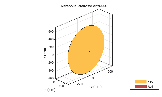
Estimate Memory Requirements
Since the parabolic reflector is an electrically large structure, it is good to estimate the amount of RAM needed to solve a given structure at the frequency of design. Use the memoryEstimate function to do this.
m = memoryEstimate(p,f)
m =
'890 MB'
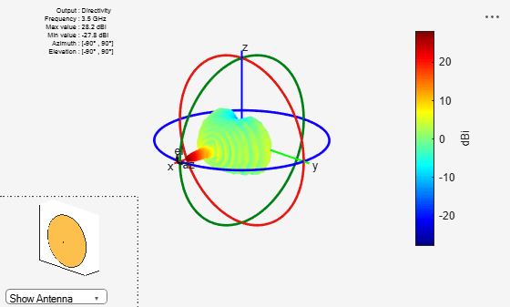
Plot 3D Radiation Pattern
Calculate the 3D far-field directivity pattern for the forward-half plane including the boresight. Additionally, rescale the magnitude to enhance the features in the pattern using the PatternPlotOptions object.
az = -90:1:90;
el = -90:1:90;
figure
pattern(p,f,az,el)
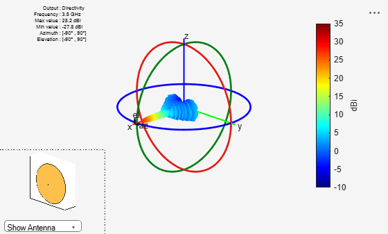
Create a PatternPlotOptions object and rescale the magnitude for the plot.
patOpt = PatternPlotOptions;
patOpt.MagnitudeScale = [-10 35];
figure
pattern(p,f,az,el,patternOptions=patOpt)
Calculate Aperture Efficiency
The maximum gain from the parabolic reflector is achieved under uniform illumination of the aperture (amplitude, phase). A feed pattern that compensates for the spherical spreading loss with the angle off from the axis and at the same time becoming zero at the rim to avoid spillover related losses would achieve this ideal efficiency of unity [2]. In reality there are different types of antennas that are used as feeds such as dipoles, waveguides, horns etc. Using the pattern analysis, you can numerically estimate the aperture efficiency. This calculation yields an aperture efficiency of approximately 50% for a dipole feed.
Dmax = pattern(p,f,0,0);
eta_ap = (10^(Dmax/10)/(pi^2))*(lambda/D)^2
eta_ap =
0.3384
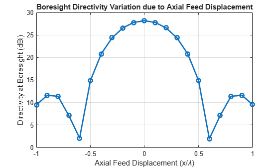
Effect of Axial Displacement of Feed
In certain applications it might be necessary to position the feed away from the focal point of the reflector. As expected such a configuration will introduce phase aberrations which will translate to a pattern degradation. Investigate the effect of an axial displacement of the feed, both - towards and away from the focus on the peak gain at boresight, i.e. (az,el) = (0,0) degrees. To do so, vary the x-coordinate of the FeedOffset property on the parabolic reflector.
feed_offset = -lambda:0.1*lambda:lambda;
Dmax_offset = zeros(size(feed_offset));
for i = 1:numel(feed_offset)
    p.FeedOffset = [feed_offset(i),0,0];
    Dmax_offset(i) = pattern(p,f,0,0);
end
figure
plot(feed_offset./lambda,Dmax_offset,'o-',LineWidth=2)
xlabel("Axial Feed Displacement (x/\lambda)")
ylabel("Directivity at Boresight (dBi)")
grid on
title("Boresight Directivity Variation due to Axial Feed Displacement");
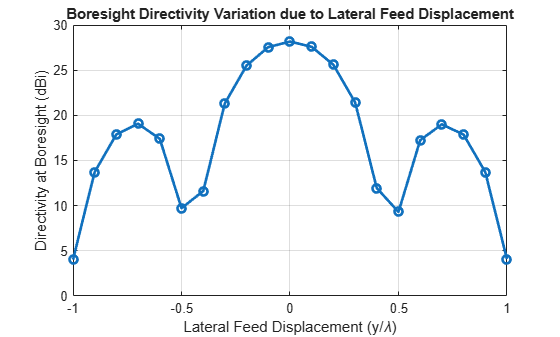
Effect of the Lateral Displacement Feed
Displacement of the feed way from the axis, laterally results in beam scan. For symmetric parabolic reflectors this effect is limited. Similar to the previous section, continue to look at the bore sight gain variation as a function of the feed being displaced along the y-axis.
Dmax_offset = zeros(size(feed_offset));
for i = 1:numel(feed_offset)
    p.FeedOffset = [0,feed_offset(i),0];
    Dmax_offset(i) = pattern(p,f,0,0);
end
figure
plot(feed_offset./lambda,Dmax_offset,'o-',LineWidth=2)
xlabel("Lateral Feed Displacement (y/\lambda)")
ylabel("Directivity at Boresight (dBi)")
grid on
title("Boresight Directivity Variation due to Lateral Feed Displacement");
Effect of Random Surface Errors on Reflector Surface
Ideally the surface of parabolic reflector is perfectly smooth without any surface imperfections. Manufacturing processes and mechanical stresses result in a surface that deviates from the perfect paraboloid. Use an RMS surface error term for each co-ordinate and analytically estimate the gain degradation due to surface errors [3].
epsilon_rms = lambda/25;
chi = (4*F_by_D)*sqrt(log(1 + 1/(4*F_by_D)^2));
Gmax_est = 10*log10(eta_ap*(pi*D/lambda)^2*exp(-1*(4*pi*chi*epsilon_rms/lambda)^2))
Gmax_est =
27.3330
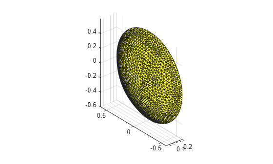
Next, build a geometric model of the reflector with surface errors. To do so, isolate the mesh for the reflector alone and perturb the points on the surface with a zero-mean Gaussian random process. The standard deviation of this process is assigned to be the RMS surface error. After perturbing the points, compute the rms surface error to confirm that the process deviation is indeed close to what we set.
p.FeedOffset = [0,0,0];
[Pt,t] = exportMesh(p);
idrad = find(Pt(:,1)>=p.FocalLength);
idref = find(Pt(:,1)<p.FocalLength);
removeTri = [];
for i = 1:size(t,1)
    if any(t(i,1)==idrad)||any(t(i,2)==idrad)||any(t(i,3)==idrad)
        removeTri = [removeTri,i];
    end
end
tref = t;
tref(removeTri,:) = [];
figure
patch(Faces=tref(:,1:3),Vertices=Pt,FaceColor="yellow");
axis equal;
axis tight;
grid on;
hfig = gcf;
ax = findobj(hfig,type="axes");
z = zoom;
z.setAxes3DPanAndZoomStyle(ax,'camera');
view(-40,30)
Create Gaussian noise for perturbing surface mesh.
n = epsilon_rms*randn(numel(idref),3);
Ptnoisy = Pt(idref,:) + n;
rms_model_error = sqrt(mean((Pt(idref,:)-Ptnoisy).^2,1))
rms_model_error = 1×3

    0.0035    0.0034    0.0034
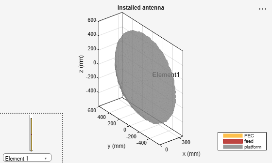
Create an STL file out of the reflector surface and make it the platform for an installed antenna analysis as shown. The excitation element is the same as before. Assign the position of the element using the feedLocation property on the parabolic reflector.
TR = triangulation(tref(:,1:3),Ptnoisy);
stlwrite(TR,"noisyref.stl")
pn = installedAntenna;
pl = platform;
exciter = p.Exciter;
exciter.Tilt = 0;
exciter.TiltAxis = [0 1 0];
pl.FileName = "noisyref.stl";
pl.Units = "m";
pn.Platform = pl;
pn.Element = exciter;
pn.ElementPosition = [p.FeedLocation(1),0,0];
figure
show(pn)
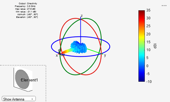
Far-field 3D Pattern for Reflector Surface with Errors
The effect of the surface errors on the reflector result in a 3 dB boresight gain reduction. This effect is particularly important to consider at the Ka, Ku and higher bands
patnOpt = PatternPlotOptions;
patnOpt.MagnitudeScale = [-10 35];
figure
pattern(pn,f,az,el,patternOptions=patnOpt)
References
[1] “Satellite Coverage Maps | Intelsat.” Accessed May 26, 2022. https://www.intelsat.com/ses-intelsat-fleetmaps/.
[2] Stutzman, Warren L., and Gary A. Thiele. Antenna Theory and Design, p. 307. 3rd ed. Hoboken, NJ: Wiley, 2013.
[3] J. Ruze, "Antenna tolerance theory—A review," in Proceedings of the IEEE, vol. 54, no. 4, pp. 633-640, April 1966, doi: 10.1109/PROC.1966.4784.