Model and Analyze Dual Polarized Patch Microstrip Antenna

This example shows how to design and measure a wideband dual polarized microstrip antenna that finds its use at the base station of a cellular system. In order to achieve the wideband characteristic, this design considers a slot coupled patch antenna structure.

Building Aperture Coupled Antenna

Define Parameters

Parameters given below defines the offsets for upper and lower slots and the stublengths.

of_1=12e-3;
of_2=-6e-3;
LM=7e-3;
LM_2=7e-3;

taken from reference page.no:55

Define Patch

In this antenna, the radiating element is patchMicrostrip. Above the patch, a dielectric substrate with EpsilonR of 3.38, acts like a radome. Below the patch there is a foam material of EpsilonR 1.025.

Lp=50e-3;
patch=antenna.Rectangle('Length',Lp,'Width',Lp,'Center',[0 0]);

Define H-shaped Slots

The double slots perform the dual polarized operation. Each slot is H-shaped and positioned on the ground plane in "T" formation. This formation provides a good isolation level among port1 and port2.

Define Upper H-shape Slot

Ls1=12e-3;
Ws1=0.5e-3;
Ls2=1e-3;
Ws2=22e-3;
f1=antenna.Rectangle('Length',Ws1,'Width',Ls1,'Center',[0 of_1]);
f2=antenna.Rectangle('Length',Ws2,'Width',Ls2,'Center',[0 of_1+(Ls1/2)+(Ls2/2)]);
f3=antenna.Rectangle('Length',Ws2,'Width',Ls2,'Center',[0 of_1-(Ls1/2)-(Ls2/2)]);
f4=f1+f2+f3;

Define Lower H-shape Slot

Ls1_2=17e-3;
Ls2_2=1e-3;
Ws1_2=0.5e-3;
Ws2_2=17e-3;
f5=antenna.Rectangle('Length',Ls1_2,'Width',Ws1_2,'Center',[0 of_2]);
f6=antenna.Rectangle('Length',Ls2_2,'Width',Ws2_2,'Center',[(Ls1_2/2)+(Ls2_2/2) of_2]);
f7=antenna.Rectangle('Length',Ls2_2,'Width',Ws2_2,'Center',[-((Ls1_2/2)+(Ls2_2/2)) of_2]);
f8=f5+f6+f7;

Define Ground Plane

Create the ground plane shape for the antenna. The ground plane in this case is a square of size 100mm x 100mm.

LGp=100e-3;
Ground_plane=antenna.Rectangle('Length',LGp,'Width',LGp,'Center',[0 0]);

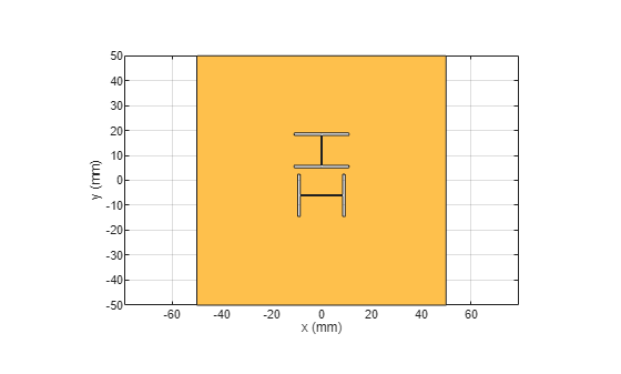
Define Slotted Ground Plane

Use the rectangle shape primitives to create the H-slots. Use the Boolean subtraction operation for slotting the Ground plane.

Gp_slot=Ground_plane-f4-f8;
figure;
show(Gp_slot);

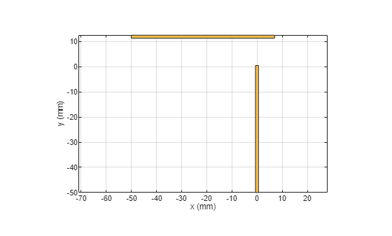
Define Feed Lines

Use a feed line of size 50mm x 1.181mm for the upper H-slot. Use a feed line of size 44mm x 1.181mm for the lower H-slot. Connect the stubs at the end of the feed lines.

L1=50e-3;
W1=1.181e-3;
L1_2=44e-3;
W1_2=1.181e-3;
feed_1=antenna.Rectangle('Length',L1,'Width',W1,'Center',[-(L1/2) of_1]);
feed_2=antenna.Rectangle('Length',W1_2,'Width',L1_2,'Center',[0 -((L1_2/2))+(of_2)]);
feed_1_2=feed_1+feed_2;
stub_1=antenna.Rectangle('Length',LM,'Width',W1,'Center',[(LM/2) of_1]);
stub_2=antenna.Rectangle('Length',W1,'Width',LM_2,'Center',[0 of_2/2]);
stub=stub_1+stub_2;
feed=feed_1_2+stub;
figure;
show(feed);

Define PCB Stack

Use the pcbStack to define the metal and dielectric layers and the feed for the aperture coupled patch antenna. The layers are defined top-down. In this case, the top-most layer is a dielectric layer. The second layer is a patch of square shape, and the third layer is another dielectric, followed by a fourth layer which is the ground plane. Fifth Layer is again the same dielectric which is used as first layer. Sixth layer is related to feed lines.

p = pcbStack;
d1=dielectric('EpsilonR',3.38,'Thickness',0.51e-3,'Name','RO4003');
d2=dielectric('EpsilonR',1.025,'Thickness',14e-3,'Name','Foam');
p.BoardThickness=d1.Thickness+d2.Thickness+d1.Thickness;
p.BoardShape.Length=LGp;
p.BoardShape.Width=LGp;
p.Layers={d1,patch,d2,Gp_slot,d1,feed};
p.FeedLocations=[-L1 of_1 4 6;0 -L1_2+of_2 4 6];
p.FeedDiameter=feed_1.Width/3;
figure;
show(p);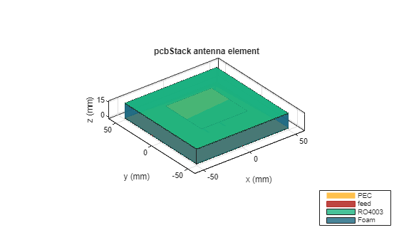

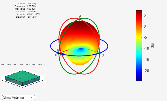
Plot Radiation Pattern

Plot the radiation pattern of the antenna at the frequencies of best match. Use a resonant frequency of 1.79 GHz to plot the radiation pattern.

figure;
pattern(p,1.79e9);

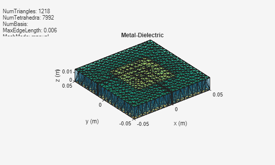
Meshing Antenna

Mesh the antenna with maximum edge length of 0.036m.

 figure;
 mesh(p,'MaxEdgeLength',0.036);

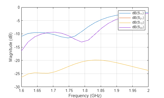
Calculate and Plot S-parameters

The plot shows return loss characteristics(S11,S22) and isolation(S12) between ports.

figure;
sf=sparameters(p,linspace(1.6e9,2e9,20));
rfplot(sf);

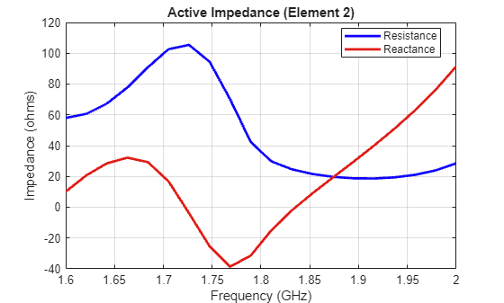
Plot Impedance Pattern

Use a frequency range from 1.5 GHz to 1.9 GHz with 20 frequency points to plot the impedance pattern.

figure;
impedance(p,linspace(1.5e9,1.9e9,20),1);

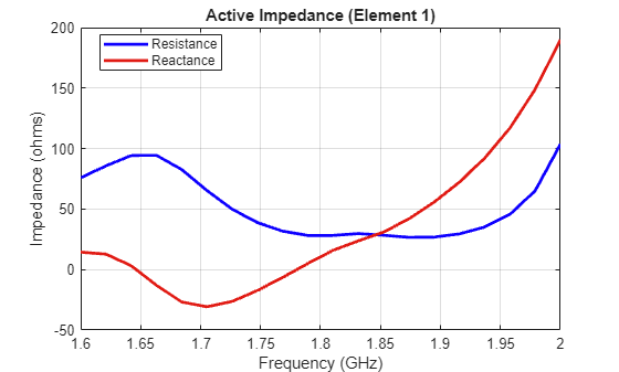
figure;
impedance(p,linspace(1.5e9,1.9e9,20),2);

Conclusion

The design and analysis of the dual polarized aperture coupled antenna using Antenna Toolbox agrees well with the referred results.

References

[1] Meltem Yildirim, "Design of Dual Polarized Wideband Microstrip Antennas", pp. 54-70.