Miniaturize Patch Antennas Using Metamaterial-Inspired Technique
This example shows how to design a miniaturized patch antenna at 2.4 GHz with a complementary split-ring resonator (CSRR) loading plane and evaluate its performance, with results as published in [1]. The antenna is miniaturized by shrinking its circular patch structure from the original radius of 23.1 mm to 6 mm.
Define Patch Dimensions
The microstrip patch in this example has 3 layers: top layer, loading plane, and ground plane. The board is a square with the side length B_d. r_0 is the original radius of the resonant patch in the top layer, which is shrunk to r. The CSRR has N complementary split rings in the loading plane, with the split width of w and the inner and outer radius of R2_in and R2_out, respectively.
clc
r_0 = 23.1e-3;
r = 14e-3;
B_d = 2.2*r_0;
N = 7;
w = 0.011*N;
R2_in = 0.3521;
R2_out = (R2_in*N/1.9079)-w;
fw = 2e-3;
Design Top Layer
Create a circular patch with the radius of r.
circle_L1 = antenna.Circle(Center = [0 0],Radius = r);
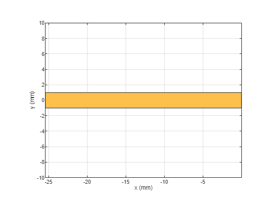
Create the feed as a rectangle.
rect_L1 = antenna.Rectangle(Length = B_d/2,Width = fw);
Move the feed in the x-y plane to connect it to the circular patch.
translate(rect_L1,[-B_d/4 0 0]);
Create a polygon combining the patch and the feed, and then plot the resulting shape.
polygon_L1 = circle_L1+rect_L1;
show(polygon_L1);
title("Top Layer")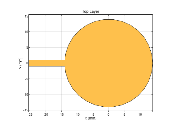
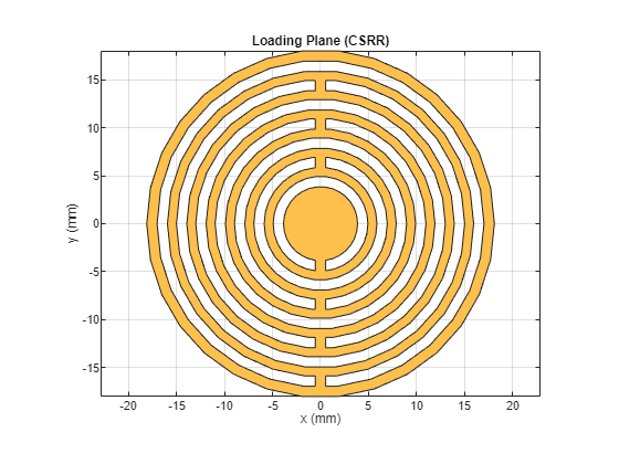
Design Loading Plane
To create a CSRR with seven rings, first, create a variable r_rad which generates multiplying factors for each of the seven rings. Then use a MATLAB for loop to iterativley add and remove circles to create the ring slots that make up the CSRR.
r_rad = linspace(R2_out,R2_in,N);
sign = -1;
circ_outer_L2 = antenna.Circle(Center = [0 0],Radius = (R2_out+w)*r);
for i = 1:length(r_rad)
    circle_Minus = antenna.Circle(Center = [0 0],Radius = r_rad(i)*r);
    circle_Plus = antenna.Circle(Center = [0 0],Radius = (r_rad(i)-w)*r);
    rect_Minus = antenna.Rectangle(Center = [0,sign*(r_rad(i)-w/2)*r],Length = w*r,Width = (w+w/1.3)*r);
    if i == 1
        spliti = circ_outer_L2-circle_Minus+circle_Plus+rect_Minus;
        CSRR_L2 = spliti;
    end
    CSRR_L2 = CSRR_L2-circle_Minus+circle_Plus+rect_Minus;
    sign = sign*-1;
end
show(CSRR_L2)
title("Loading Plane (CSRR)")
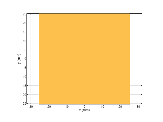
Design Ground Plane
Design the ground plane as a rectangle with the same dimension as that of the board.
rect_L3 = antenna.Rectangle(Length = B_d,Width = B_d);
show(rect_L3)
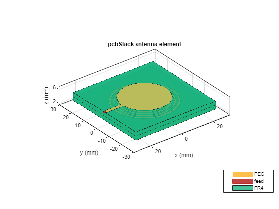
Design Board
Define the shape of the board and create the stack with the layers mentioned above and specified dielectric layers in between.
boardShape = antenna.Rectangle(Length = B_d,Width = B_d);
Create PCB stack using previously defined layers and two dielectric layers.
p = pcbStack;
p.BoardShape = boardShape;
d1 = dielectric("FR4");
% d1 = dielectric("RT5870");
d1.Thickness = 2.34e-3;
% d2 = dielectric("RT5870");
d2 = dielectric("FR4");
d2.Thickness = 2.34e-3;
p.BoardThickness = d1.Thickness+d2.Thickness;
p.Layers = {polygon_L1,d1,CSRR_L2,d2,rect_L3};
p.FeedLocations = [-B_d/2 0 1 5];
p.FeedDiameter = fw/2;
figure
show(p)
Analyze Performance of Miniature Antenna
Before evaluating the board's performance, estimate the memory required to solve the mesh structure. You can do this by using the memory estimator.
memoryEstimate(p,2.6e9)
ans =
'2.8 GB'
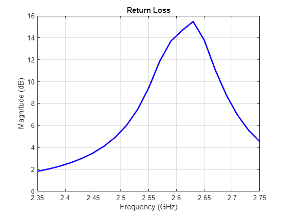
Compute Return Loss
This example uses the following commenteefine code to compute the return loss of the designed patch antenna.
[~] = mesh(p,'MaxEdgeLength',0.03,'MinEdgeLength',0.005);
freq = linspace(2.35e9,2.75e9,21);
figure;
returnLoss(p, freq);
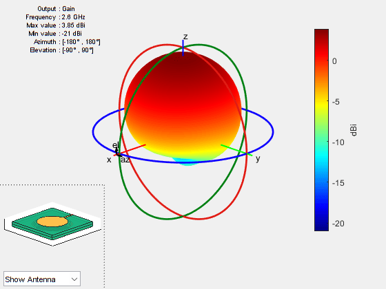
Plot Radiation Pattern
Plot the 3-D radiation pattern of the patch.
figure;
pattern(p,2.6e9)
Visualize the current density of the patch.
figure;
current(p,2.396e9,scale = "log")
Reference
[1] Ouedraogo, Raoul O., Edward J. Rothwell, Alejandro R. Diaz, Kazuko Fuchi, and Andrew Temme. “Miniaturization of Patch Antennas Using a Metamaterial-Inspired Technique.” IEEE Transactions on Antennas and Propagation 60, no. 5 (May 2012): 2175–82. https://doi.org/10.1109/TAP.2012.2189699.