Modeling and Simulation of an Autonomous Underwater Vehicle
This example shows how to simulate the dynamics and control of an autonomous submarine using Simulink® and the Aerospace Blockset™. Given a reference position/velocity, this example designs a control law enabling the autonomous submarine to obey the reference parameters.
Examples of the use of autonomous underwater vehicles include deep-sea geological surveying, exploration, and search and rescue. Autonomizing these vehicles saves the weight of a human crew, reducing the overall mission cost and increasing the scope of mission objectives (for example, enabling large sample returns or enabling more fuel to be stored on board, which can lead to a longer mission duration).
For the purposes of this example, all motion is performed via propulsion, without the use of control surfaces.
This example uses this workflow of the autonomous submarine - given a set of reference parameters (either a target position or velocity), and sensor-measured values of the vehicle's current velocity and position, the controller calculates appropriate thrust commands to pass to the plant for actuation. After the plant implements a thruster control input, sensors pass information about the new position and velocity of the submarine to a noise filter and then to the controller to determine the next set of thrust commands required for the vehicle to obey the reference parameters.
Modeling Assumptions
Assume that the submarine is cuboidal in shape, with a mass of 10 kg and a volume of 0.01 m^3. For underwater propulsion, the vehicle uses thrusters of two different sizes, rated at 5 and 10 pound-force of thrust (T5 and T10). In total, the vehicle uses five thrusters arranged as follows: - Two T10 Thrusters to allow for forward/backward motion, referred to as surge. - Two T5 Thrusters to allow for sideways motion, referred to as sway. - One T10 Thruster to allow for upward/downward motion, referred to as heave.
Assume that all thrusters in a group operate identically. For example, the two T10 thrusters intended to provide surge always provide identical amounts of thrust at any given instant of time. This means that they cannot be individually commanded to produce different thrusts. In addition, this simulation does not model any weight changes.
Assume that the submarine is always fully submerged in the water. This means that the vehicle does not resurface and therefore no component of the vehicle interacts with air above the water.
Open the Model
open_system("asbAUV");

The top level diagram closely resembles the high-level workflow presented in the introduction.
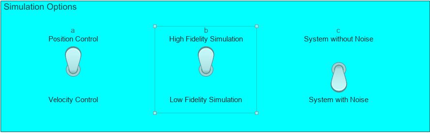
The model presents three simulation options: - The type of control, in this case position or velocity. - The fidelity of the simulation with respect to the modeling of the environmental forces. A high fidelity simulation involves a more accurate computation of the lift and drag generated by the submarine. A low fidelity involves a less accurate computation. - The presence of noise in the sensor measurements.
Control Strategy
The "Translational Reference" subsystem contains the reference parameters for the vehicle to follow. The Signal Editor block generates these parameters. The model passes these parameters and the sensor measurements of the vehicle's actual position and velocity to the translational controller.
open_system("asbAUV/Translation Controller")
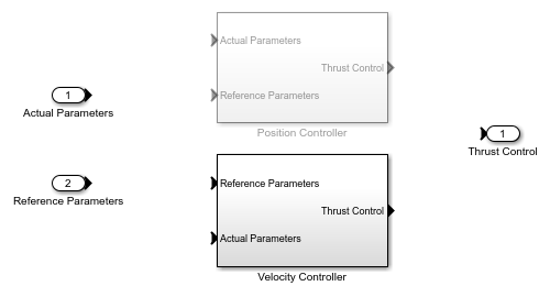
Depending on the selection in the top-level diagram, either the position controller or the velocity controller is activated. The "Position Controller" subsystem uses one PID controller block to determine the required thrust command in each direction, requiring three controller blocks in total.
open_system("asbAUV/Translation Controller/Position Controller")
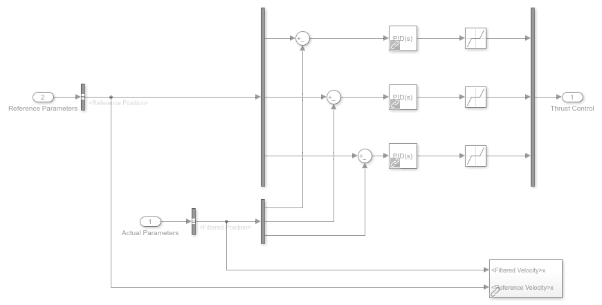
The resulting thrust commands are then passed through dead zone blocks to discard values of thrust control that are less than 0.05.
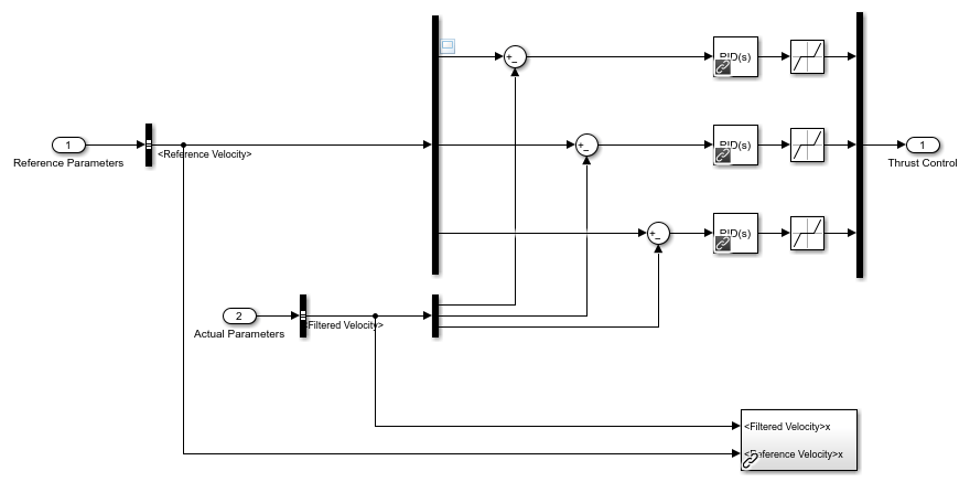
The "Velocity Controller" subsystem also uses three PID controller blocks to determine the required thrust commands.
open_system("asbAUV/Translation Controller/Velocity Controller")
Vehicle and Environment Modeling
The computed thrust commands are then passed to the "Plant and Environment Model" subsystem.
open_system("asbAUV/Plant and Environment Model")

In the "Plant and Environment Model" subsystem, the computed thrust commands are first passed to the "Propulsion Forces and Moments" subsystem, which converts these thrust commands into Pulse-Width Modulated (PWM) signals using a 1D Lookup Table block. The subsystem then converts the PWM signals into resultant thrust forces using the transfer functions of the thrusters.
These resultant thrust forces are then used to compute the resulting moments on the vehicle.
To compute the hydrodynamic (lift and drag) and hydrostatic (weight and buoyancy) forces, the "Environmental Forces and Moments" subsystem accepts the vehicle angle of attack, sideslip angle, velocity in the body frame, and the Euler orientation angles relative to the inertial frame as inputs.
open_system("asbAUV/Plant and Environment Model/Environmental Forces & Moments")
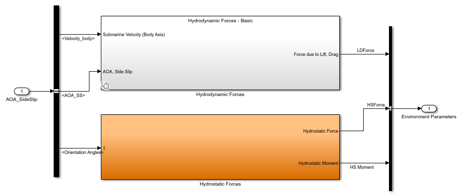
The "Hydrodynamic Forces" subsystem contains two conditionally operated subsystems, "Hydrodynamic Forces - Accurate" and "Hydrodynamic Forces - Basic".
open_system("asbAUV/Plant and Environment Model/Environmental Forces & Moments/Hydrodynamic Forces")

The selected level of simulation fidelity determines the subsystem that gets activated.
- High Fidelity Simulation: The "Hydrodynamic Forces - Accurate" subsystem becomes activated and the computation of lift and drag takes into account the effects caused by the angle of attack and the sideslip angle on the classic lift/drag equation.
- Low Fidelity Simulation: The "Hydrodynamic Forces - Basic" subsystem becomes activated and the computations of lift and drag do not consider these effects and only use the classic lift/drag equations.
Regardless of the chosen level of simulation fidelity, each subsystem performs lift and drag computations in separate subsystems.
In the "Hydrodynamic Forces - Basic" subsystem, the computation of drag assumes a drag coefficient, CD, of 0.75. Note that the signals for angle of attack and sideslip angles are ignored.
open_system("asbAUV/Plant and Environment Model/Environmental Forces & Moments/Hydrodynamic Forces/Hydrodynamic Forces - Basic/Marine Drag - Body Axes")
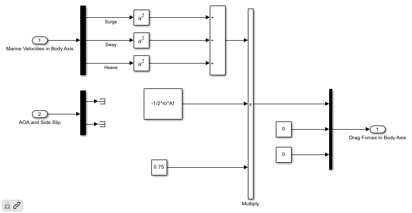
The net result is given by:

Where: - A_frontal represents the frontal area, assumed to be 0.001 m^2. - V represents the vehicle's velocity. - rho represents the density of the water. - CD represents the coefficient of drag.
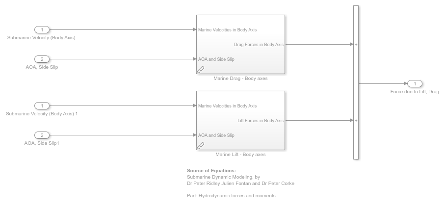
The computation of lift is performed using the same equation with a lift coefficient of 0.2 and assuming the same frontal area.
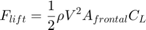
If a high-fidelity simulation is selected, the "Hydrodynamic Forces - Accurate" subsystem becomes activated. This selection also componentizes the computation of lift and drag into their own subsystems.
open_system("asbAUV/Plant and Environment Model/Environmental Forces & Moments/" + ...
    "Hydrodynamic Forces/Hydrodynamic Forces - Accurate")
Note that in the "Force Exerted due to Drag (Body axis)" subsystem, the angle of attack and sideslip angles are now used.
open_system("asbAUV/Plant and Environment Model/Environmental Forces & Moments" + ...
    "/Hydrodynamic Forces/Hydrodynamic Forces - Accurate/Marine Drag - Body axes")
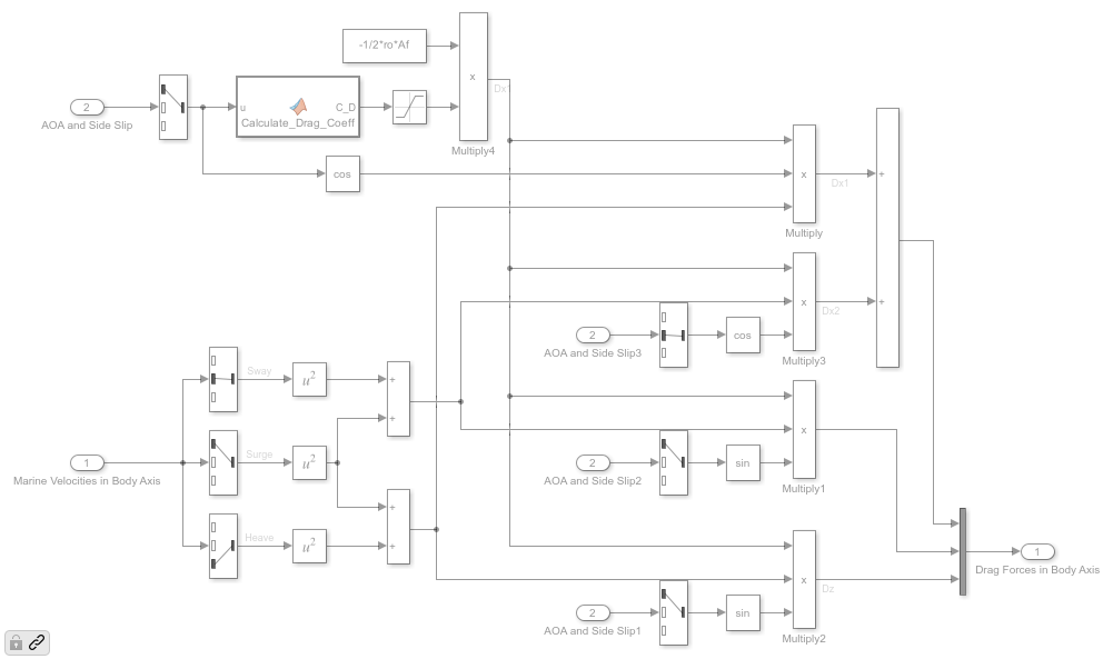
Letting alpha represent the angle of attack, beta represent the side-slip angle, Vx, Vy, and Vz represent surge, sway, and heave respectively, drag is computed as:
![$$F_{drag} = \frac{1}{2} \rho A_{f} C_{D} [(V_{x}^{2} + V_{y}^{2)}) \sin(\beta) + (V_{x}^{2} + V_{z}^{2}) \sin(\alpha) + (V_{y}^{2} + V_{z}^{2}) \cos(\alpha) + (V_{x}^{2} + V_{y}^{2}) \cos(\beta)]$$](../examples/aeroblks/win64/AutonomousUnderwaterVehicleExample_eq12468979539960736407.png)
The drag coefficient is computed as a function of angle of alpha as follows.

Similarly, the accurate computation of lift also considers the effects of angle of attack. Side-slip angle does not affect the generated lift because the example is only concerned with the vertical component of force generated due to forward motion. This computation occurs in the "Force Exerted due to lift (Body axis)" subsystem.
open_system("asbAUV/Plant and Environment Model/Environmental Forces & Moments/Hydrodynamic Forces/Hydrodynamic Forces - Accurate/Marine Lift - Body axes");

The net result is given by:

For small angles, the coefficient of lift varies linearly with angle of attack.
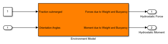
Simultaneously, the hydrostatic force and moment (due to the vehicle's weight on buoyancy) are computed inside the "Hydrostatic Forces" subsystem.
open_system("asbAUV/Plant and Environment Model/Environmental Forces & Moments/Hydrostatic Forces")
The computed hydrodynamic, hydrostatic, and previously computed propulsion forces and moments are passed to the "Combine Forces and Moments" subsystem, which vectorially adds all the forces and moments to be passed to the "Dynamics Solver" subsystem, whose contents are pictured below. The subsystem accepts the total forces and moments as inputs. It outputs the vehicle velocity, position, angle of attack, side-slip angle, orientation angles, angular rates, and accelerations after applying the previously computed thrust input.
open_system("asbAUV/Plant and Environment Model/Dynamics solver")

For organizational purposes, the velocity, position, angle of attack, side-slip angle, orientation angles, and their rates are grouped into a bus signal labelled "AUV Data". The orientation angles, angle of attack, side-slip angle, and velocity in the body frame are grouped into another bus signal called "Internal Parameters".
The AUV Data signal is passed onto the subsystem "Sensor Data and State Estimation" (see top level diagram), while the internal parameters are fed back to the "Environmental Forces and Moments" subsystem to compute the total force and moment resulting from the hydrodynamic and hydrostatic forces at the next time step.
Sensor Data and State Estimation
The aim of the "Sensor Data and State Estimation" subsystem is to mimic a sensor measurement and demonstrate the use of filters to remove noise by introducing noise into the vehicle's current motion parameters.
open_system("asbAUV/Sensor data and State Estimation")
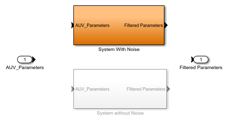
Your decision on the inclusion of noise is reflected in the subsystem that is activated. If you want to simulate without noise, the AUV parameters are passed through this subsystem with no modification. Conversely, if you decide to simulate with the presence of noise, the "System With Noise" subsystem is activated.
open_system("asbAUV/Sensor data and State Estimation/System With Noise");

The AUV data (comprising the vehicle's accelerations, angular rates, angular accelerations, and center of gravity location) and the gravitational constant are passed to the Three-axis Inertial Measurement Unit block, which generates noisy measurements of the vehicle acceleration and angular rates. A Mux block combines these signals into a single signal called "IMU Measurements", which is passed to the "Internal Filter" subsystem.
open_system("asbAUV/Sensor data and State Estimation/System With Noise/Internal filter")
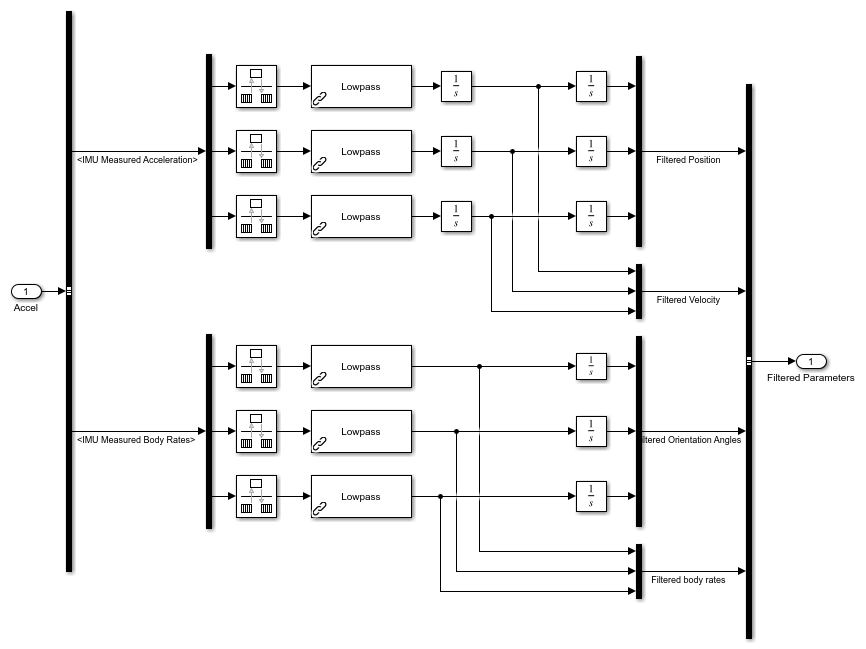
The IMU Measurements signal is separated back into measured acceleration and measured angular rates. Each quantity has three components (x, y, and z) which are passed through a lowpass filter to obtain a best estimate of the relevant quantity. These components are integrated over time to obtain filtered quantities of the vehicle's position, velocity, orientation angles, and angular rates in the body frame.
These filtered quantities are then passed into the "Translation Controller" subsystem to compute the required thrust commands for the next time step.
Why use the Aerospace Blockset?
Hand-modeling six coupled equations of motion in Simulink is prone to errors. To reduce the chance of modeling errors arising from this, use the 6DOF block from the Aerospace Blockset. The 6DOF block computes the following position data, given the total force and moment acting on a body:
- Vehicle velocity in the flat Earth frame - Vehicle position in the flat Earth frame - Euler rotation angles - The direction cosine matrix relating the body frame to the flat Earth frame - Vehicle velocity in the body-fixed frame - Angular velocity of the vehicle in the body-fixed frame - Rate of change of angular velocity (angular acceleration) in the body- fixed frame - Translational acceleration in the body-fixed axes - Translational acceleration with respect to the inertial frame
The above outputs are in different reference frames, which may not be ideal for some applications. To ensure that quantities remain in desired reference frames, use the rotation and coordinate transformation blocks.
For convenience, convert Euler rotation angles to direction cosine matrix elements and vice versa. To achieve this, use the Direction Cosine Matrix to Rotation Angles and Rotation Angles to Direction Cosine Matrix blocks.
The Three-axis Inertial Measurement Unit block is useful in the state estimation part of the problem. Given the vehicle's actual acceleration, angular rates, angular accelerations, center of gravity location, and the acceleration due to gravity, the block mimics an IMU and outputs measured values of the vehicle's acceleration and angular rates.
The Aerospace Blockset also lets you simulate a 6DOF system in which the vehicle's mass is variable. This capability lets you model fuel consumption as the simulation runs, resulting in a more accurate model. Other available functionalities include actuators, aerodynamics simulations, instrument modeling, center of gravity estimation, etc.
Simulation - Position Control
For the purposes of this simulation, the vehicle's position is controlled in a high-fidelity simulation with noise present in the measurements of the vehicle's current parameters. The simulation time is set at 300 seconds.
Looking at the reference parameters for position, the X and Y coordinates of the final position are specified to be -10. The Z coordinate of the reference position remains at zero until 150 seconds into the simulation, at which time it changes to 5 meters. This is implemented via a Step function block.
Start out by setting the switches to the desired positions.
Then, click the 'Run' button or press Ctrl+T. After compilation, the model starts to run and a figure window showing the live orientation and position of the vehicle is opened. At 150 seconds of simulation time, the vehicle can be seen translating upwards, consistent with the reference parameters for position provided in the "Translational Reference subsystem". Furthermore, the thrust inputs can be verified via the thrust input gauges located below the switches on the top-level diagram.

After the simulation completes, a second figure window opens which plots the trajectory history of the vehicle in three dimensions. From here, it can be verified that the vehicle's motion satisfies the reference parameters provided.

Alternate Control Strategies
The control problem illustrated by this example can be further extended to be an optimal control problem. In other words, as opposed to merely controlling the position and velocity of the vehicle, the controller must now control the position and velocity while simultaneously satisfying another set of constraints. For example, keeping the vehicle on a known path while minimizing fuel consumption. In view of this, two alternate control strategies can be used, model predictive control and linear quadratic regulator.
Model Predictive Control
Using a model predictive controller, a finite time-horizon is computed. For each time step leading up to the horizon, the optimal control input for the current time step is computed (via linearizing the model at the current time step), actuated, and then reoptimized to the new time-horizon until the end of the simulation. The main advantage of this control strategy over PID is that the optimization of the control input required for the current time step takes into consideration the future time steps. Furthermore, this enables the controller to anticipate future events and effect appropriate control measures. This control strategy is particularly useful if the vehicle is to automatically detect and avoid obstacles.
Linear Quadratic Regulator
A linear quadratic regulator (LQR) is also a good candidate for a control strategy in such an optimal control problem. Using an LQR involves computing the optimal control inputs that minimize a specified quadratic cost function. In this specific problem, the cost function can be the amount of fuel used that must be minimized. The difference between this and model predictive control is that an LQR optimizes over the entire time horizon of the simulation, while an MPC uses a receding horizon. An advantage of LQR over MPC lies in the lower amount of computational power required.
See Also
6DOF (Euler Angles) | Direction Cosine Matrix to Rotation Angles | Rotation Angles to Direction Cosine Matrix | Three-axis Inertial Measurement Unit
Select a Web Site
Choose a web site to get translated content where available and see local events and offers. Based on your location, we recommend that you select: United States.
You can also select a web site from the following list
Americas
- América Latina (Español)
- Canada (English)
- United States (English)
Europe
- Belgium (English)
- Denmark (English)
- Deutschland (Deutsch)
- España (Español)
- Finland (English)
- France (Français)
- Ireland (English)
- Italia (Italiano)
- Luxembourg (English)
- Netherlands (English)
- Norway (English)
- Österreich (Deutsch)
- Portugal (English)
- Sweden (English)
- Switzerland
- United Kingdom (English)
Asia Pacific
- Australia (English)
- India (English)
- New Zealand (English)
- 中国
- 日本Japanese (日本語)
- 한국Korean (한국어)