Hohmann Transfer with the Spacecraft Dynamics Block

This example shows how to model a Hohmann transfer of a spacecraft between two circular coplanar orbits in Simulink® and visualize the transfer in a satellite scenario. It uses:

• Aerospace Blockset™ Spacecraft Dynamics block

• Aerospace Blockset Attitude Profile block

• Aerospace Toolbox satelliteScenario object

The Aerospace Blockset Spacecraft Dynamics block models translational and rotational dynamics of spacecraft using numerical integration. To represent thrust from the propulsion system and the moments generated by the attitude controller, you can configure the block to accept propellant mass flow rate, exhaust velocity, and body moments. To implement the Hohmann transfer, perform the necessary maneuvers by applying the necessary moments to orient the spacecraft in the desired direction and applying thrust to achieve the necessary delta-v.

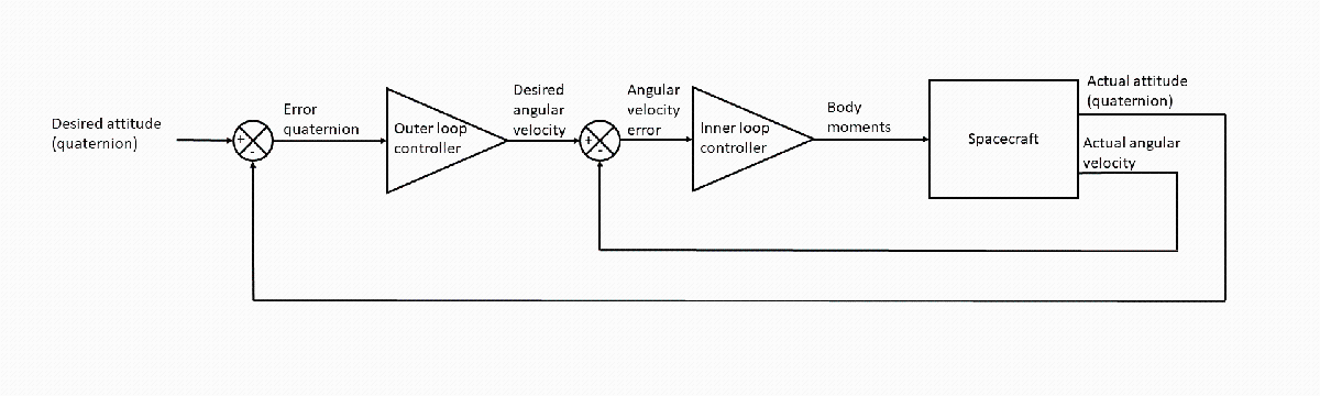
The attitude controller consists of the Aerospace Blockset Attitude Profile block, which returns the shortest quaternion rotation that aligns the spacecraft's provided alignment axis with the specified target. This quaternion constitutes the alignment error, which is corrected by a cascade controller. The inner loop of the controller controls the angular velocity. The outer loop of the controller controls the attitude. Both loops involve a simple proportional controller. In this example, the spacecraft's x-axis (assumed to be the thrust axis) is commanded to align with the desired delta-v direction.

The Aerospace Toolbox satelliteScenario object lets you load previously generated, time-stamped ephemeris and attitude data into a scenario from a timeseries or timetable object. This data is interpolated in the scenario object to align with the scenario time steps, allowing you to incorporate data generated in a Simulink model into either a new or existing satelliteScenario object. In this example, the Spacecraft Dynamics block computes the satellite orbit and attitude states. For visualization on the satellite scenario viewer, this data is then used to add a satellite to a new satelliteScenario object.

The Hohmann Transfer

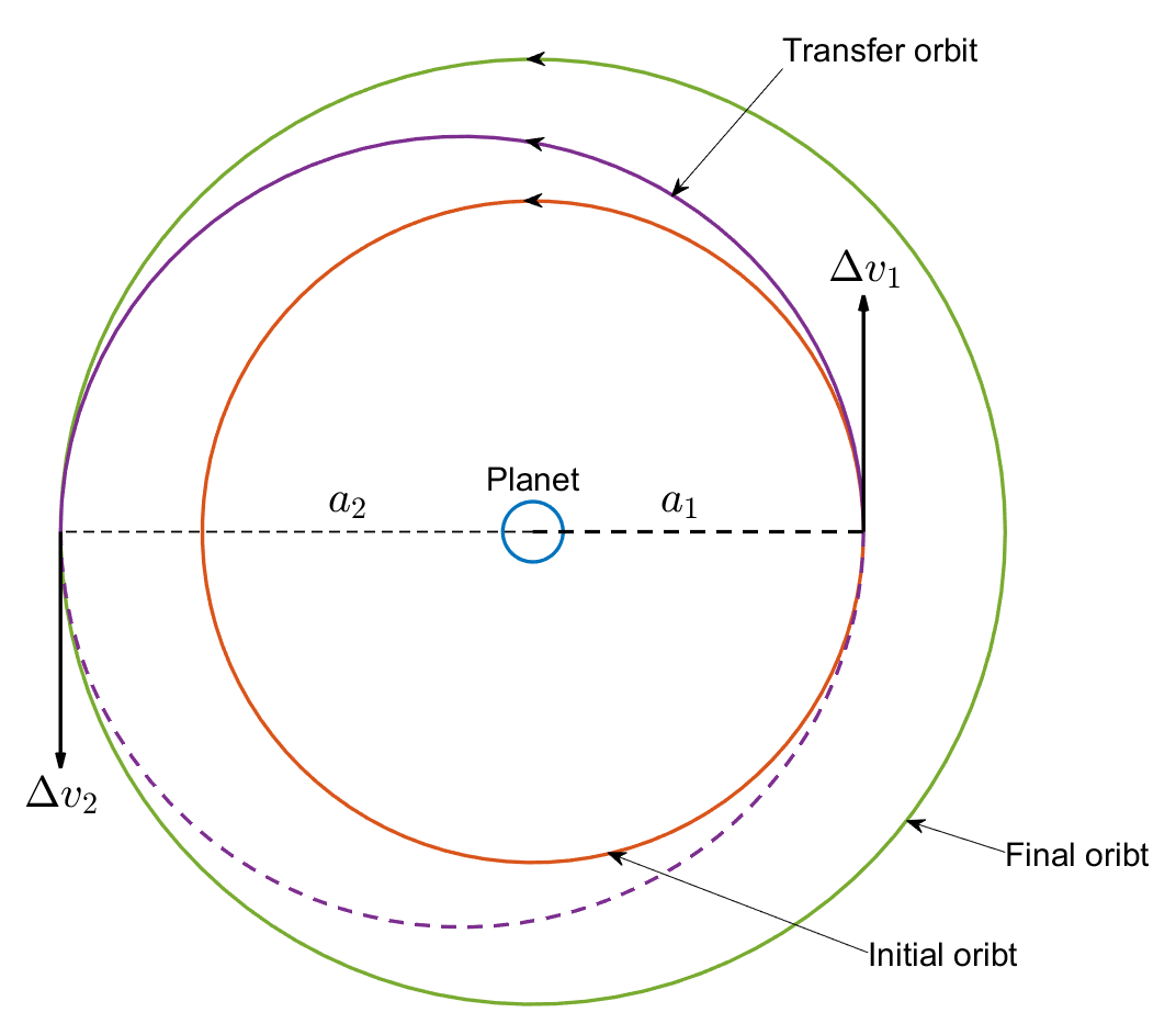
The Hohmann transfer consists of two coplanar maneuvers to transfer a spacecraft between two orbits that lie on the same plane. The initial and final orbits can be circular or elliptical. In this example, the orbits are assumed to be circular. The transfer orbit is an ellipse tangential to the two orbits. The transfer involves two maneuvers:

• The first maneuver at the tangent point of the initial orbit (the first transfer point) places the spacecraft on the elliptic transfer orbit.

• The second maneuver at the tangent point of the final orbit (the second transfer point) inserts the spacecraft into this orbit.

The transfer angle, the angle between the position vector of the spacecraft at the two transfer points with respect to the planet, is 180 degrees. Because the transfer ellipse is tangential, the required velocity change (delta-v) at the transfer points is the difference between the circular orbital speed and the velocity on the elliptic transfer orbit at the transfer points. The direction of the delta-v is the tangent at the transfer points.

The following figure illustrates a Hohmann transfer between two coplanar circular orbits. If the second maneuver is not performed, the spacecraft follows the dashed magenta back to the first tangent point.

Suppose $a_1$ and $a_2$ are the orbital radii of the initial and final circular orbits. The semimajor axis of the transfer orbit is given by:

$$a_T=\frac{(a_1+a_2)}{2}$$

The velocity magnitude at any given point on the initial circular orbit is given by:

$$v_1=\sqrt{\frac{\mu }{a_1}}$$

where $$\mu$$ is the standard gravitational parameter of the planet (Earth). The velocity on the transfer orbit at the first transfer point is derived from the following energy equation:

$$\frac{v_{T,1}^2}{2}-\frac{\mu }{a_1}=-\frac{\mu }{2a_T}$$

where $$v_{T,1}$$ is the velocity on the transfer orbit at the first transfer point (the tangent between the initial orbit and the transfer orbit). Therefore:

$$v_{T,1}=\sqrt{2\mu (\frac{1}{a_1}-\frac{1}{2a_T})}$$

Consequently, the delta-v at the first transfer point ($\Delta v_1$) is given by:

$$\Delta v_1=v_{T,1}-v_1$$

The direction of $\Delta v_1$ is the tangent at the first transfer point on the initial orbit, as illustrated above. Similarly, the delta-v at the second transfer point ($\Delta v_2$) can be calculated as follows:

$$\begin{array}{l}{v}_2=\sqrt{\frac{\mu }{a_2}}\\ v_{T,2}=\sqrt{2\mu (\frac{1}{a_2}-\frac{1}{2a_T})}\\ \Delta v_2=v_2-v_{T,2}\end{array}$$

As before, the direction of $\Delta v_2$ is the tangent at the second transfer point on the final orbit. The time taken to coast from the first transfer point to the second (transfer duration) is half the orbital period of the transfer orbit.

$$t_T=\pi \sqrt{\frac{a_T^3}{\mu }}$$

Mission Overview

The mission begins on December 14, 2022, 1:04 AM UTC. Define this time as a datetime object and a Julian date.

initialTime = datetime(2022,12,14,1,4,0);
initialTimeJD = juliandate(initialTime);

At the initial time, the spacecraft is in a circular orbit with the following specifications:

• Semimajor axis ($$a_1$$) = 7,000 km

• Eccentricity = 0

• Inclination = 45 degrees

• Right ascension of ascending node = 90 degrees

• Argument of periapsis = 30 degrees

• True anomaly = 0 degrees

Set the semimajor axis, a1, of the initial orbit in meters.

a1 = 7000e3;

Set the eccentricity, e1, of the initial orbit.

e1 = 0;

Set the inclination, i1, of the initial orbit in degrees.

i1 = 45;

Set the right ascension of ascending node, raan1, of the initial orbit in degrees.

raan1 = 90;

Set the argument of periapsis, w1, of the initial orbit in degrees.

w1 = 30;

Set the true anomaly, theta1, of the initial orbit in degrees.

theta1 = 0;

Define the standard gravitational parameter for Earth in m^3/s^2.

mu = 398600.4418e9;

The spacecraft stays on the initial orbit for one full period before initiating the transfer. Calculate the time corresponding to the first transfer point, t1, in seconds.

t1 = 2*pi*sqrt((a1^3)/mu);

The spacecraft must transfer to a coplanar circular orbit with an orbital radius of 10,000 km. Accordingly, set the semimajor axis, a2, of the final orbit in meters.

a2 = 10000e3;

Calculate the semimajor axis of the transfer orbit in meters.

aTransfer = (a1 + a2)/2;

The second transfer point occurs exactly one-half transfer orbital period after the first transfer point. Accordingly, calculate the transfer duration, tTransfer, in seconds.

tTransfer = pi*sqrt((aTransfer^3)/mu);

Calculate the time corresponding to the second transfer point, t2, in seconds.

t2 = t1 + tTransfer;

The mission ends after one orbital period on the final orbit. Accordingly, define the mission end time, t2, in seconds.

tf = t2 + (2*pi*sqrt((a2^3)/mu));

Calculate Maneuvers

The maneuvers at the first and second transfer points are defined by the maneuver times, delta-v magnitude, and delta-v direction. The maneuver times (t1 and t2) are calculated in the previous topic. The remaining parameters are calculated in this topic.

Calculate Delta-V Magnitudes

Calculate the circular velocity on the initial orbit.

v1 = sqrt(mu/a1);

Calculate the velocity on the transfer orbit at the first transfer point.

vTransfer1 = sqrt(2*mu*((1/a1) - (1/(2*aTransfer))));

Calculate the delta-v magnitude at the first transfer point.

deltav1 = vTransfer1 - v1;

Calculate the circular velocity on the final orbit.

v2 = sqrt(mu/a2);

Calculate the velocity on the transfer orbit at the second transfer point.

vTransfer2 = sqrt(2*mu*((1/a2) - (1/(2*aTransfer))));

Calculate the delta-v magnitude at the second transfer point.

deltav2 = v2 - vTransfer2;

Calculate Delta-V Directions

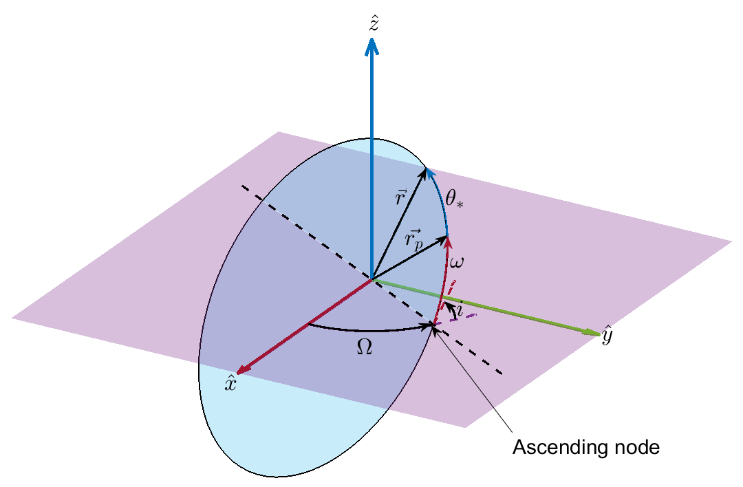
For circular orbits, the velocity direction in three-dimensional space is given by:

$$\underset{}{\overset{ˆ}{\text{v}}}=(-\cos \Omega \sin (\omega +{\theta }_{*})-\sin \Omega \cos i\cos (\omega +{\theta }_{*}))\underset{}{\overset{ˆ}{x}}+(-\sin \Omega \sin (\omega +{\theta }_{*})+\left(\cos \Omega \cos i\cos (\omega +{\theta }_{*})\right))\underset{}{\overset{ˆ}{y}}+\sin i\cos (\omega +{\theta }_{*})\underset{}{\overset{ˆ}{z}}$$

where:

• $$\underset{}{\overset{ˆ}{\text{v}}}$$ is the velocity direction.

• $$\Omega$$ is the right ascension of ascending node.

• $$i$$ is the inclination.

• $$\omega$$ is the argument of periapsis.

• $${\theta }_{*}$$ is the true anomaly.

These quantities are defined in the International Celestial Reference Frame (ICRF) spanned by $$\underset{}{\overset{ˆ}{x}}$$, $$\underset{}{\overset{ˆ}{y}}$$, and $$\underset{}{\overset{ˆ}{z}}$$ axes, as illustrated below.

Notes:

• The velocity vector is always tangential to the orbit. Because the transfer orbit is tangential to the initial and final circular orbits at the transfer points, the velocity directions on the circular and transfer orbits at these points are the same.

• The first transfer point is at the periapsis of the transfer orbit. The second transfer point is at the apoapsis of the transfer orbit. Therefore, the true anomalies on the transfer orbit corresponding to these transfer points are 0 degrees and 180 degrees respectively.

• Because the initial and final orbits are coplanar, the transfer orbit is also coplanar with these orbits. Therefore, the right ascension of ascending node and inclination are the same as those of the initial and final orbits.

• Because the true anomaly on the initial orbit corresponding to the first transfer point is the same as that on the transfer orbit (0 degrees), the argument of periapsis of the transfer orbit is the same as that of the initial orbit.

Define the true anomaly at the first transfer point on the transfer orbit in degrees.

thetaStar = 0;

Calculate the delta-v direction at the first transfer point.

deltav1Direction = [- cosd(raan1)*sind(w1 + thetaStar) - sind(raan1)*cosd(i1)*cosd(w1 + thetaStar); ...
    - sind(raan1)*sind(w1 + thetaStar) + cosd(raan1)*cosd(i1)*cosd(w1 + thetaStar); ...
    sind(i1)*cosd(w1 + thetaStar)];

Define the true anomaly at the second transfer point on the transfer orbit in degrees.

thetaStar = 180;

Calculate the delta-v direction at the second transfer point.

deltav2Direction = [- cosd(raan1)*sind(w1 + thetaStar) - sind(raan1)*cosd(i1)*cosd(w1 + thetaStar); ...
    - sind(raan1)*sind(w1 + thetaStar) + cosd(raan1)*cosd(i1)*cosd(w1 + thetaStar); ...
    sind(i1)*cosd(w1 + thetaStar)];

Calculate Burn Durations

The preceding equations assume impulsive maneuvers, wherein the delta-v is achieved instantaneously. To approximate an impulsive delta-v in Simulink, assume a large thrust acceleration. The thrust for a given propellant mass flow rate $$\underset{}{\overset{\dot{}}{m}}$$ and specific impulse $$I_{sp}$$ is given by:

$$T=\underset{}{\overset{\dot{}}{m}}{g}_0{I}_{sp}$$

where $$g_0$$ is the acceleration due to gravity of the Earth equator. The quantity $$g_0{I}_{sp}$$ is the exhaust velocity, $$v_e$$. Then, to approximate the impulsive delta-v, assume a propellant mass flow rate of 500 kg/s, a specific impulse of 400 s, and an initial spacecraft mass m0 of 1000 kg. These assumptions create a thrust acceleration of 1962 m/s^2 (or 200 gs) when the propellant is full. This acceleration increases as the propellant gets depleted. The high thrust acceleration reduces the time required to achieve the calculated delta-v.

g0 = 9.81;
Isp = 400;
ve = g0*Isp;
mDot = 500;
m0 = 1000;

Based on the above thrust parameters, calculate the burn durations for each delta-v maneuver using the rocket equation. The rocket equation shows how the spacecraft mass (hence, the propellant mass) changes for a given delta-v. Suppose the initial spacecraft mass is $$m_0$$ and the mass after applying a delta-v of $$\Delta v$$ reduces the mass to $$m_1$$. $$m_0$$ and $$m_1$$ are related by this rocket equation:

$$\frac{m_0}{m_1}=e^{\left(\frac{\Delta v}{v_e}\right)}$$

Calculate the mass m1 after the maneuver at the first transfer point.

m1 = m0/exp(deltav1/ve);

Calculate the burn duration in seconds for the maneuver at the first transfer point.

burnDuration1 = (m0-m1)/mDot;

Calculate the mass m2 after the maneuver at the second transfer point.

m2 = m1/exp(deltav2/ve);

Calculate the burn duration in seconds for the maneuver at the second transfer point.

burnDuration2 = (m1-m2)/mDot;

The burn durations are about 0.3 s and 0.24 s for the first and second transfer point, respectively. Next, examine the Simulink model that simulates the Hohmann transfer using the calculated maneuver parameters.

Examine Model

Examine the model that simulates the Hohmann transfer in Simulink by implementing the calculated maneuver parameters.

Open the Example Model

Open the model. At the top level, the model consists of the Maneuver, Attitude controller, and Spacecraft subsystems.

model = 'hohmannTransfer';
open_system(model);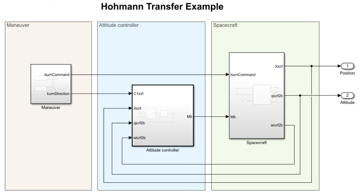

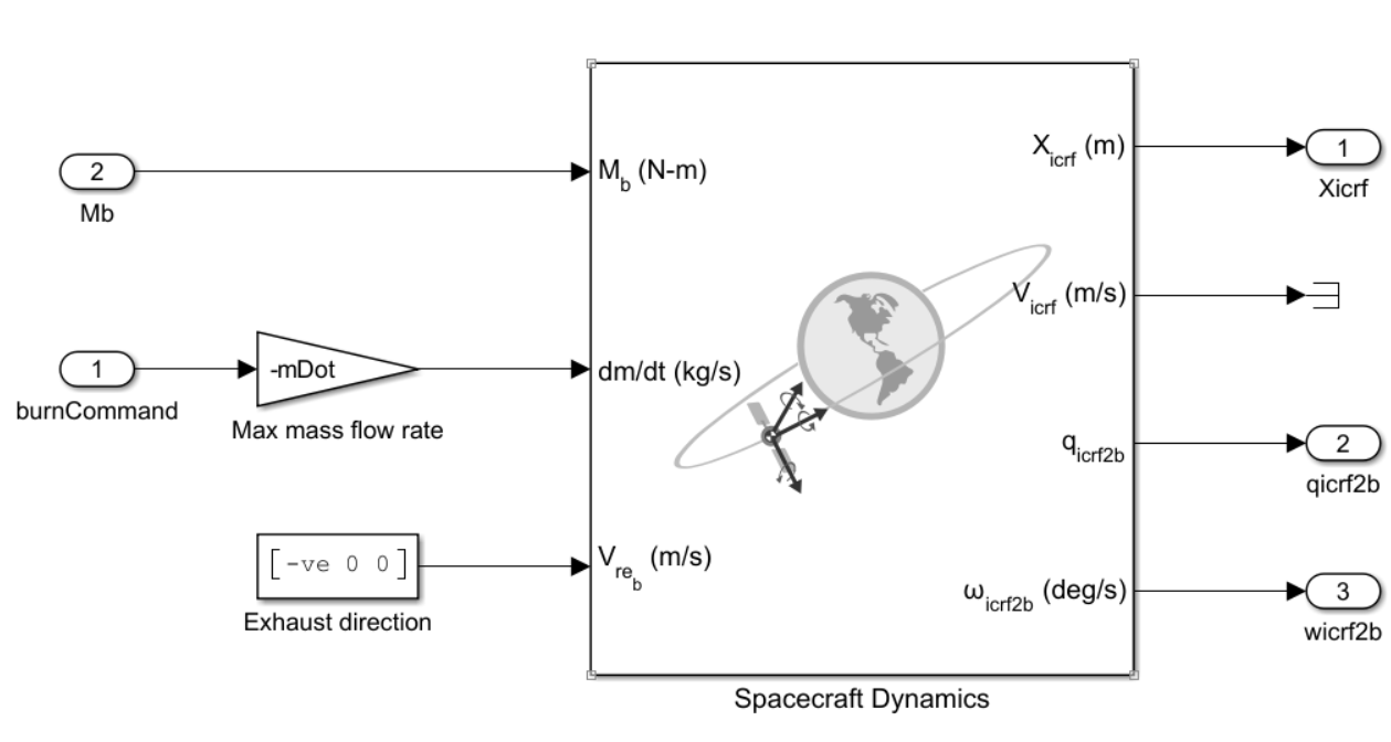
Spacecraft Subsystem

The Spacecraft subsystem models the spacecraft motion using the Spacecraft Dynamics block. The block accepts the external body moments, mass flow rate, and exhaust velocity as inputs. It outputs the ICRF position, attitude with respect to ICRF, and angular velocity in the body frame. The ICRF velocity output is unused.

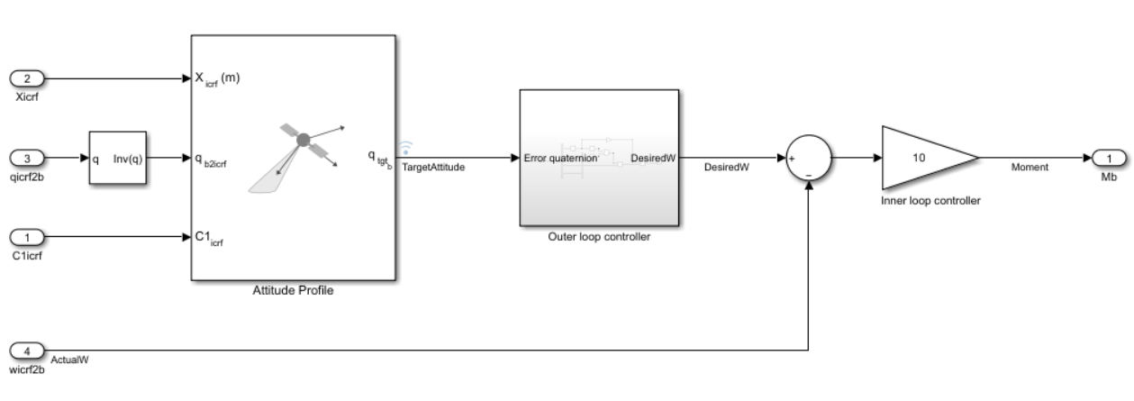
Attitude Controller Subsystem

The attitude controller subsystem calculates the body moments to align the x-axis of the spacecraft body (the primary alignment vector) with the burn direction (the primary constraint vector) for each maneuver and the z-axis of the spacecraft (the secondary alignment vector) with the z-axis of ICRF. The alignment of the primary vectors must be exact. This requirement implies that the exact alignment of the secondary vectors is not always possible. The goal in this instance is to minimize the misalignment of the secondary vectors.

The high-level architecture of the controller is given here. It is a cascade controller, where the inner loop controls the angular velocity, and the outer loop controls the attitude.

The Attitude controller subsystem implementing the above architecture is shown here.

The Outer loop controller subsystem is shown here.

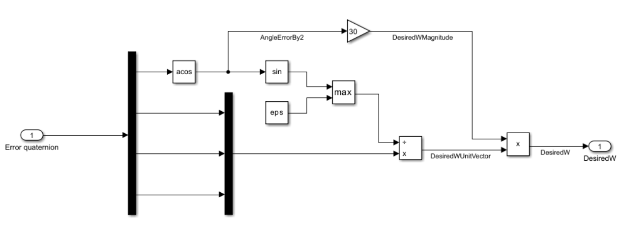
This controller extracts the rotation axis and angle from the error quaternion. The goal is to drive this angle to 0. A proportional controller calculates the angular velocity magnitude required to drive this angle to 0. The rotation axis calculated from the error quaternion is the desired unit angular velocity vector. This unit vector, combined with the desired angular velocity magnitude, constitutes the desired angular velocity vector, which in turn drives the inner loop.

The inner loop compares the desired angular velocity vector output from the outer loop controller against the actual angular velocity vector. The angular velocity error is fed to the inner loop controller, which is also implemented as a proportional controller. The output of this controller is the desired body moment vector, which is input to the Spacecraft Dynamics block in the Spacecraft subsystem.

Maneuver Subsystem

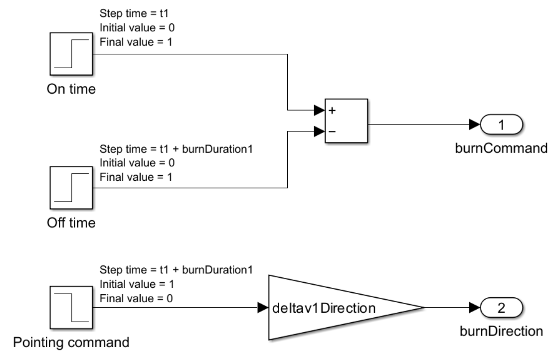
The Maneuver subsystem generates the burn commands (burnCommand) and burn direction (burnDirection) for the maneuvers at the transfer points. The Transfer orbit injection subsystem generates the burn command and direction for the first transfer point. The Orbit circularization subsystem generates the same for the second transfer point.

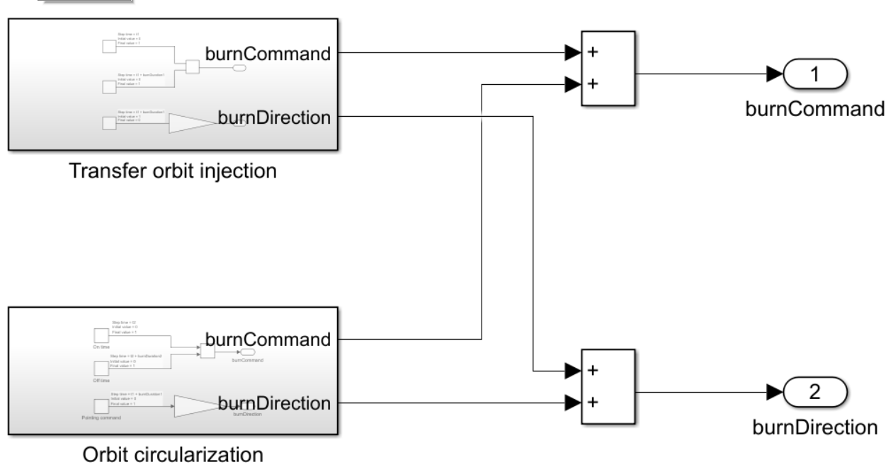
The burn commands take values 0 or 1. When the value is 1, the spacecraft propulsion system generates thrust. The burnCommand output drives the dm/dt input of the Spacecraft Dynamics block through the Max mass flow rate block in the Spacecraft subsystem. The burnCommand must equal 1 between t1 and t1 + burnDuration1 corresponding to the maneuver at the first transfer point and between t2 and t2 + burnDuration2 corresponding to the maneuver at the second transfer point. At all other times, it must equal 0.

The burn direction must initially equal the delta-v direction at the first transfer point (burnDirection1). After the first maneuver is complete (at t1 + burnDuration1), the burn direction must equal the delta-v direction at the second transfer point (burnDirection2) and maintain this direction for the duration of the simulation. The burnDirection output drives the Attitude controller subsystem.

The switching logic for the burnCommand and burnDirection implemented by the Transfer orbit injection subsystem is illustrated here.

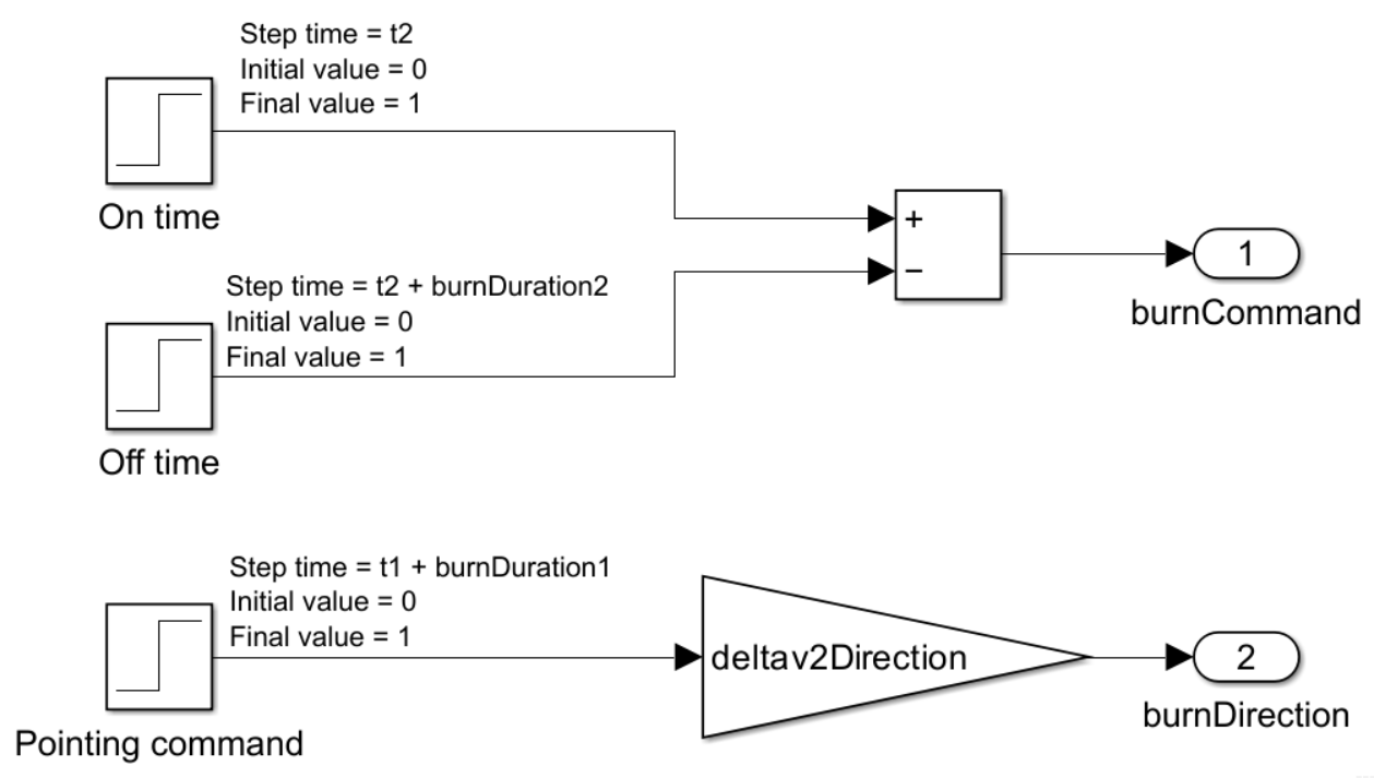
The switching logic for the burnCommand and burnDirection implemented by the Orbit circularization subsystem is illustrated here.

Run Simulation

Run the simulation with the sim function. The model is configured to run in Rapid Accelerator mode for performance.

simOut = sim(model);

### Building the rapid accelerator target for model: hohmannTransfer
### Successfully built the rapid accelerator target for model: hohmannTransfer

Build Summary

Top model rapid accelerator targets built:

Model            Action                        Rebuild Reason                                    
=================================================================================================
hohmannTransfer  Code generated and compiled.  Code generation information file does not exist.  

1 of 1 models built (0 models already up to date)
Build duration: 0h 1m 4.0375s

Extract Position and Attitude

Extract the position and attitude timeseries from the simulation results and convert them to timetables. These timetables will be imported into a satellite scenario object for visualizing the mission.

positionTT = timeseries2timetable(simOut.yout{1}.Values);
attitudeTT = timeseries2timetable(simOut.yout{2}.Values);

Visualize Mission

Import the simulation results into a satellite scenario to visualize the mission on a satellite scenario viewer.

Create a Satellite Scenario Object

Create a satellite scenario object based on the initial time and simulation duration. Set the sample time to 60 seconds.

startTime = initialTime;
stopTime = startTime + seconds(tf);
sampleTime = 60;
sc = satelliteScenario(startTime,stopTime,sampleTime);

Add a Satellite to the Scenario

Add a satellite to the scenario using the position timetable.

sat = satellite(sc,positionTT,Name = "Spacecraft");

Define Attitude Profile Based on Simulation

Use pointAt to define the attitude profile of the satellite in the scenario based on the attitude timetable.

pointAt(sat,attitudeTT);

Launch Satellite Scenario Viewer

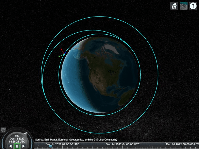
Launch a satellite scenario viewer to visualize the scenario. Set the camera reference frame to Inertial to inertially fix the camera orientation. Left-click and hold anywhere inside the satellite scenario viewer window to pan the camera. Adjust the zoom level using the scroll wheel.

% Launch a satellite scenario viewer
v = satelliteScenarioViewer(sc,CameraReferenceFrame = "Inertial");

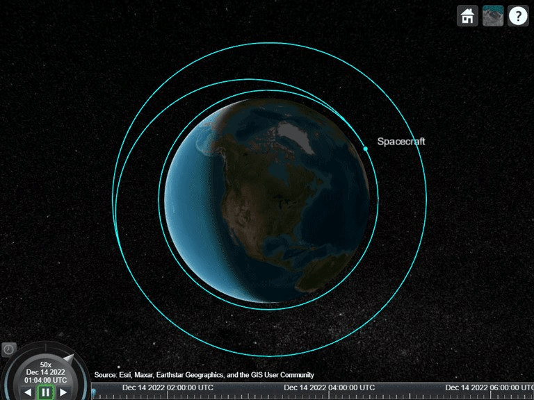
The viewer shows the trajectory flown by the spacecraft. The initial orbit, the transfer orbit, and the final orbit are clearly visible.

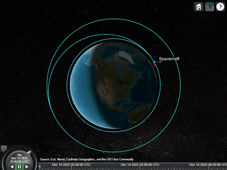
Visualize Body Coordinate Axes

Use coordinateAxes to visualize the body coordinate axes of the spacecraft. This enables you to visualize the attitude of the spacecraft. The red, green, and blue arrows are the body x-, y-, and z-axes respectively.

coordinateAxes(sat);

Play Scenario

Animate the scenario using play.

play(sc);

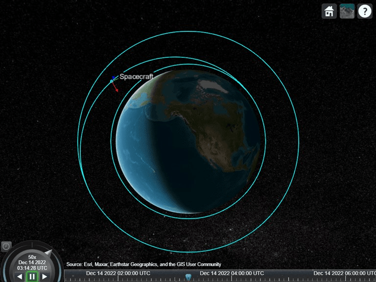
Note how the spacecraft attitude changes in preparation for the first maneuver that occurs after one orbital period.

v.CurrentTime = sc.StartTime + seconds(t1/3);

After the first maneuver, the spacecraft reorients in preparation for the second maneuver.

v.CurrentTime = sc.StartTime + seconds(t1 + 2000);

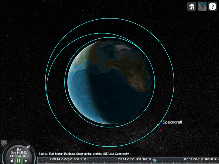
After the second maneuver, the spacecraft is on the final orbit. It continues to hold the same attitude used during the second maneuver.

v.CurrentTime = sc.StartTime + seconds(t2 + 3000);

Conclusion and Next Steps

This example demonstrates how to model Hohmann transfer using the Spacecraft Dynamics block and visualize the trajectory using satellite scenario. Of note:

• The initial and final orbits are assumed to be circular and coplanar, which result in a transfer orbit that is also coplanar.

• The spacecraft attitude is controlled for each maneuver in the transfer using an attitude controller. This controller uses the Attitude Profile block to calculate the error between the desired attitude and the actual attitude.

• The maneuvers are calculated assuming impulsive delta-v's, where the desired velocity change is assumed to be achieved instantaneously.

• The Simulink model approximates the impulsive delta-v by allowing the spacecraft to generate a large amount of thrust, reducing the burn durations.

• The thrust is modeled using the specific impulse and propellant mass flow rate.

To improve the example:

• Model finite burns by using a more realistic propellant mass flow rate. A finite burn results in a final orbit that is slightly different than the desired orbit unless the maneuver calculations are updated to accommodate such burns. Such calculations incorporate optimal control theories and involve numerical methods as opposed to analytical methods.

• Model reaction thrusters and use the calculated control moments to determine the control allocation among the thrusters.

• Assume elliptical initial and final orbits. Note that the transfer orbit must still be tangential to the two orbits. However, the true anomalies on the transfer orbit at the two transfer points might not be 0 and 180 degrees.