Concurrent Execution with Simulink Real-Time and Multicore Target Hardware

Running a high-fidelity plant model in real time for hardw­are-in-the-loop (HIL) simulation helps reduce the need for hardware prototypes, which, in turn, reduces development time and cost. The higher the fidelity of the model, however, the greater the risk of a CPU overrun—overloading the CPU of the target computer.

You can reduce this risk by using concurrent execution.  In concurrent execution the model is partitioned, and each part is executed in parallel on a multicore machine. By balancing out the computational load across the multiple cores of the target computer, concurrent execution improves real-time system performance because it increases the amount of code that can run within a specified sample time.

Using a model of an electric vehicle as an example, this article describes a workflow for concurrent execution using Simulink Real-Time™ and a Speedgoat dual-core target computer.

We will begin by running the model on a single core to obtain a baseline measure of real-time performance. We’ll then configure the model to utilize multiple cores and run a concurrent execution. A comparison of the single-core and multicore simulation results will show us whether there is any risk of a CPU overrun.

The High-Fidelity Plant Model

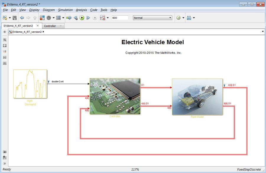
In this example we will be using an electric vehicle model built with Simulink^®, SimDriveline™, SimElectronics^®, and Simscape™ (Figure 1).

The model includes the following parts:

• Test input – the drive cycle (for this test, the US06 drive cycle)
• Operator and power management subsystem
• Battery, electric drive, and vehicle model

The goal is to be able to run this high-fidelity plant model on the HIL simulator so that we can connect a real ECU to the simulator and test its performance.

Running a Baseline Simulation

We begin by running the electric vehicle model on a single-core real-time machine to obtain the total execution time (the computation time required to execute the model in real time). We will use the execution time as a baseline for comparing the results of single-core and multicore execution.

To configure the model for Simulink Real-Time we do the following:

1. Select the solver and the sample step time—in this case, the discrete solver and Ts = 0.001.
2. Set the system target file in the Configuration Parameters>Code Generation options to “slrt.tlc.”
3. In the Configuration Parameters>Code Generation>Verification> Code Profiling option, enable “Measure task execution time” and select the save option “All measurement and analysis data.”

After this we build and download the model to the real-time machine and run it for 10 seconds. We then generate a code execution profiling report using the following command:

% Matlab Code- 
profileInfo.modelname = 'EVdemo_4_RT'; % your model name 
profData = profile_xpc(profileInfo);

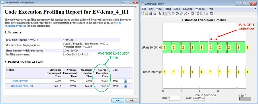
The profiling report displays a summary of model execution time (Figure 2).

For the baseline model, all the blocks are grouped as a single task during code generation. As a result, the profiling report shows only two tasks: timer interrupt and base rate.

The right-hand side of the report shows that the average execution time for the model task is 0.948 ms while the time needed to service the timer interrupt that triggers the model execution is ~ 0.003 ms.

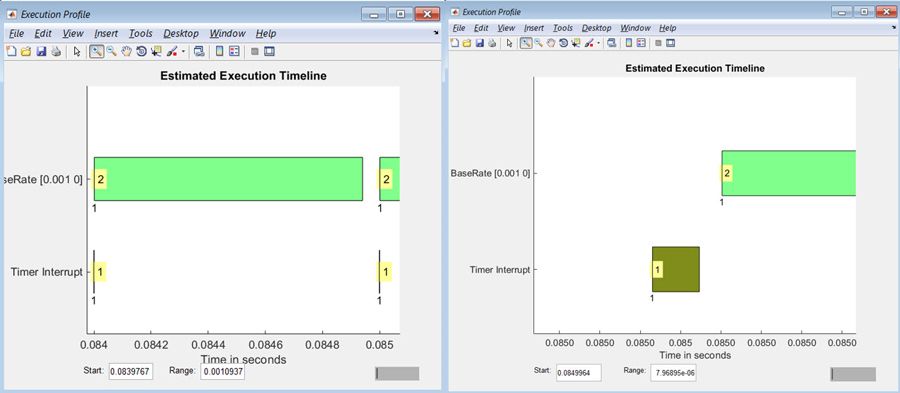
The Execution profile shows that the tasks are being executed sequentially (Figure 3).

The total execution time is the sum of the time required to service the timer interrupt and the time required to execute the model—in this example,  0.948+0.003 =~0.951 millisecond. This means that we have already used more than 95% of the core capacity. Any changes in the execution time caused by the model dynamics will lead to a CPU overrun and stop the simulation. To prevent this from happening we will use concurrent execution.

Partitioning the Model for Concurrent Execution

If the model has multiple rates, you can utilize the multiple cores of the target hardware by enabling the “Allow tasks to execute concurrently on target” option in the configuration parameters without restructuring the model. Depending on how much computational work is being done within each rate, this may or may not lead to execution time benefits. Since this step requires minimal configuration, it is an easy experiment to try. In our example, the whole model runs at a single rate, and so we will have to explicitly partition the model in order to derive the benefit of multiple cores.

There are many ways to partition a model. At a high level, the model partitioning can be based on any of the following:

• Rate – partitioning based on the multiple execution rates within the model (such as Slow rate, Fast rate)
• Physics – partitioning based on the physical characteristics of the subsystems (such as engine model, transmission model, and electrical systems)
• Functionality – separating I/O channels and plant model components

Since the test model is single-rate and we aren’t using any I/O channels, we have partitioned the model based on physical characteristics, as follows:

• Mechanical components – the vehicle model
• Electrical components – the battery model and the DC/DC converter
• Controls – the operator model

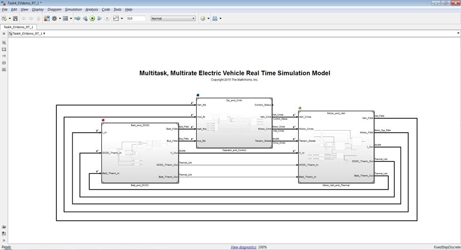
In the explicitly partitioned model, each top-level block must use the model reference block from the Simulink Ports and subsystems library (Figure 4). Using model references allows us to separate tasks at the model level.

Configuring the Model for Concurrent Execution

To configure the model for concurrent execution, we do the following:

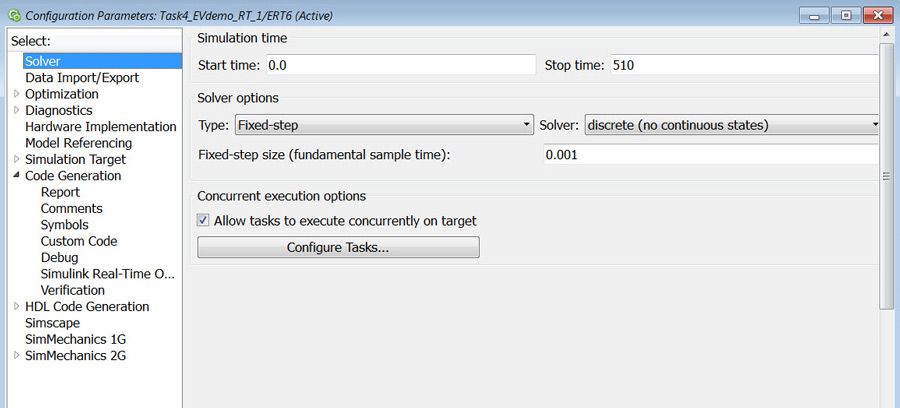
1. Under the solver settings in the Configuration Parameters dialog box, enable “Allow tasks to execute concurrently on target” and select “Configure Tasks” (Figure 5).

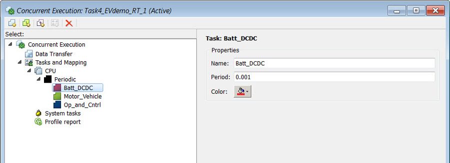
2. Create three separate tasks so that we can assign each referenced model to an individual task by clicking the Add task button on the left-hand corner of the panel (Figure 6).

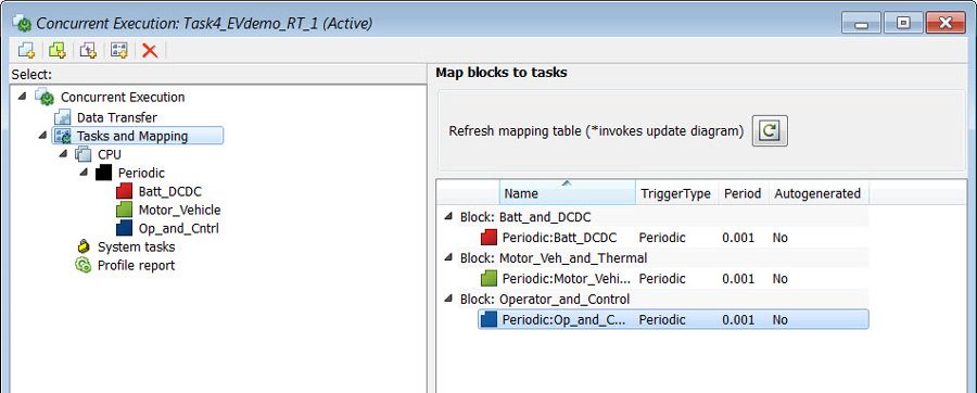
3. Assign the respective referenced models by using the Task and Mapping tab (Figure 7).

The model is now configured to utilize multiple cores. When the model is updated, the assigned tasks show up as colored icons on the top left-hand side. This means that we can always see the task assignment by looking at the top-level model.

Note that assigning tasks in this fashion changes the behavior of the simulation model by adding unit delays at the boundaries between tasks. Concurrent execution lets you see these changes via annotations on the task transition lines. It also allows you to simulate the changed behavior. During model partitioning it’s a good idea to simulate the system frequently, since unit delays can lead to changes in the functionality of the plant model.

Using the ‘Build and Download’ button we download the model to the Speedgoat real-time target computer.

Concurrent Execution Results

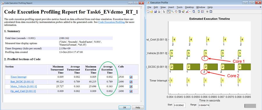
After executing the model for 10 seconds, we generate a new profiling report (Figure 8).

The report confirms that the model execution has been split into three tasks rather than the single task of the baseline model, and that the tasks are being executed in parallel. There is also an entry for the additional timer interrupt task.

We see that the average execution time for the Battery_DCDC task is the highest. This means that, from a computational perspective, this subsystem is taking up most of the execution time: 0.789 ms out of the 0.948 ms as seen in the baseline model.

Since the model tasks are now being scheduled in parallel, the total time required for the model execution is only 0.789+ 0.002 =~ 0.791— 16.82 % lower than the original 0.951 ms.

It should be noted that utilizing two cores doesn’t automatically improve performance by 50%. The actual performance improvement depends on the type of model and the way the tasks are partitioned. In addition, data transfer between multiple cores takes time, and so there is a penalty associated with creating additional tasks. More tasks allow us to split the model across multiple cores, which is good, but utilizing multiple cores also increases the overhead required for inter-core communication. For further improvements, we could use a high-performance quad-core target computer from Speedgoat instead of a dual-core machine.

In summary, concurrent execution lets you execute high-fidelity plant models in real time by utilizing the multiple cores of the target computer. We saw a significant reduction in total execution time, and that gave us sufficient assurance that the real-time execution will not stop because of CPU overruns. Reducing model execution time is beneficial in the case of HIL testing because it means we can test the controller against a higher fidelity plant model, which is a closer representation of the actual physical system.