gscatter
Scatter plot by group
Syntax
Description
gscatter(___,
fills in marker interiors. "filled")gscatter ignores this option
for markers that do not have interiors.
Examples
Scatter Plot with Default Settings
Load the carsmall data set.
load carsmallPlot the Displacement values on the x-axis and the Horsepower values on the y-axis. gscatter uses the variable names as the default labels for the axes. Group the data points by Model_Year.
gscatter(Displacement,Horsepower,Model_Year)

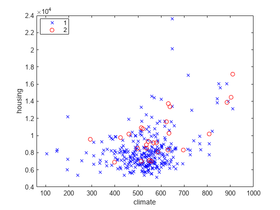
Scatter Plot with One Grouping Variable
Load the discrim data set.
load discrimThe data set contains ratings of cities according to nine factors such as climate, housing, education, and health. The matrix ratings contains the ratings information.
Plot the relationship between the ratings for climate (first column) and housing (second column) grouped by city size in the matrix group. Choose different colors and plotting symbols for each group.
gscatter(ratings(:,1),ratings(:,2),group,'br','xo')
xlabel('climate')
ylabel('housing')
Scatter Plot with Multiple Grouping Variables
Load the hospital data set.
load hospitalPlot the ages and weights of the hospital patients. Group the patients according to their gender and smoker status. Use the o symbol to represent nonsmokers and the * symbol to represent smokers.
x = hospital.Age;
y = hospital.Weight;
g = {hospital.Sex,hospital.Smoker};
gscatter(x,y,g,'rkgb','o*',8,'on','Age','Weight')
legend('Location','northeastoutside')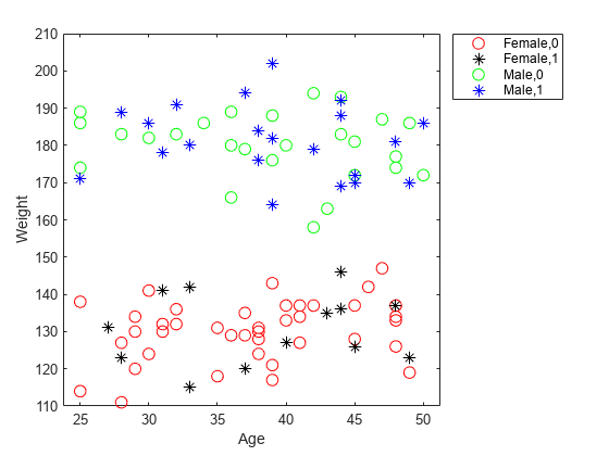
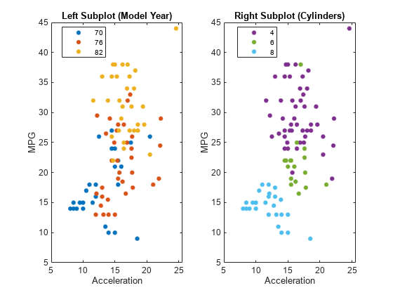
Specify Axes for Scatter Plot
Load the carsmall data set. Create a figure with two subplots and return the axes objects as ax1 and ax2. Create a scatter plot in each set of axes by referring to the corresponding Axes object. In the left subplot, group the data using the Model_Year variable. In the right subplot, group the data using the Cylinders variable. Add a title to each plot by passing the corresponding Axes object to the title function.
load carsmall
color = lines(6); % Generate color values

ax1 = subplot(1,2,1); % Left subplot
gscatter(ax1,Acceleration,MPG,Model_Year,color(1:3,:))
title(ax1,'Left Subplot (Model Year)')

ax2 = subplot(1,2,2); % Right subplot
gscatter(ax2,Acceleration,MPG,Cylinders,color(4:6,:))
title(ax2,'Right Subplot (Cylinders)')
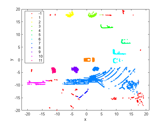
Specify Marker Colors
Specify marker colors using the colormap determined by the hsv function.
Load the Lidar scan data set which contains the coordinates of objects surrounding a vehicle, stored as a collection of 3-D points.
load('lidar_subset.mat')
loc = lidar_subset;
To highlight the environment around the vehicle, set the region of interest to span 20 meters to the left and right of the vehicle, 20 meters in front and back of the vehicle, and the area above the surface of the road.
xBound = 20; % in meters
yBound = 20; % in meters
zLowerBound = 0; % in meters
Crop the data to contain only points within the specified region.
indices = loc(:,1) <= xBound & loc(:,1) >= -xBound ...
    & loc(:,2) <= yBound & loc(:,2) >= -yBound ...
    & loc(:,3) > zLowerBound;
loc = loc(indices,:);
Cluster the data by using dbscan with pairwise distances.
D = pdist2(loc,loc);
idx = dbscan(D,2,50,'Distance','precomputed');
Visualize the resulting clusters as a 2-D group scatter plot by using the gscatter function. By default, gscatter uses the seven MATLAB default colors. If the number of unique clusters exceeds seven, the function cycles through the default colors as needed. Find the number of clusters, and generate the corresponding number of colors by using the hsv function. Specify marker colors to use a unique color for each cluster.
numGroups = length(unique(idx));
clr = hsv(numGroups);
gscatter(loc(:,1),loc(:,2),idx,clr)
xlabel('x')
ylabel('y')
Create and Modify Scatter Plot
Load the carbig data set.
load carbigCreate a scatter plot comparing Acceleration to MPG. Group data points based on Origin.
h = gscatter(Acceleration,MPG,Origin)
h =
  7x1 Line array:

  Line    (USA)
  Line    (France)
  Line    (Japan)
  Line    (Germany)
  Line    (Sweden)
  Line    (Italy)
  Line    (England)
Display the Line object corresponding to the group labeled (Japan).
jgroup = h(3)
jgroup =
  Line (Japan) with properties:

              Color: [0.9290 0.6940 0.1250]
          LineStyle: 'none'
          LineWidth: 0.5000
             Marker: '.'
         MarkerSize: 15
    MarkerFaceColor: 'none'
              XData: [15 14.5000 14.5000 14 19 18 15.5000 13.5000 17 14.5000 16.5000 19 16.5000 13.5000 13.5000 19 21 16.5000 19 15 15.5000 16 13.5000 17 17.5000 17.4000 17 16.4000 15.5000 18.5000 16.8000 18.2000 16.4000 14.5000 ... ] (1x79 double)
              YData: [24 27 27 25 31 35 24 19 28 23 27 20 22 18 20 31 32 31 32 24 26 29 24 24 33 33 32 28 19 31.5000 33.5000 26 30 22 21.5000 32.8000 39.4000 36.1000 27.5000 27.2000 21.1000 23.9000 29.5000 34.1000 31.8000 38.1000 ... ] (1x79 double)

  Use GET to show all properties
Change the marker color for the Japan group to black.
jgroup.Color = 'k';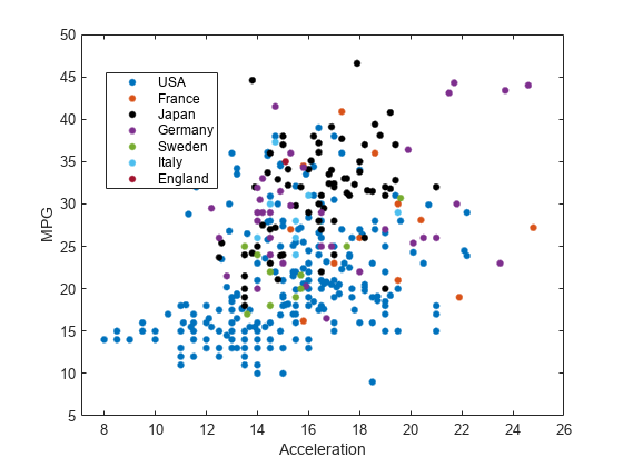
Input Arguments
x — x-axis values
numeric vector
x-axis values, specified as a numeric vector. x must
have the same size as y.
Data Types: single | double
y — y-axis values
numeric vector
y-axis values, specified as a numeric vector. y must
have the same size as x.
Data Types: single | double
g — Grouping variable
categorical vector | logical vector | numeric vector | character array | string array | cell array of character vectors | cell array
Grouping variable, specified as a categorical vector, logical vector,
numeric vector, character array, string array, or cell array of character
vectors. Alternatively, g can be a cell array
containing several grouping variables (such as {g1 g2
g3}), in which case observations are in the same group if they
have common values of all grouping variables. Points in the same group
appear on the scatter plot with the same marker color, symbol, and
size.
The number of rows in g must be equal to the length
of x.
Example: species
Example: {Cylinders,Origin}
Data Types: categorical | logical | single | double | char | string | cell
clr — Marker colors
MATLAB® default colors (default) | character vector or string scalar of short color names | matrix of RGB triplets
Marker colors, specified as a character vector or string scalar of short color names or a matrix of RGB triplets.
For a custom color, specify a matrix of RGB triplets. An RGB triplet is a
three-element row vector whose elements specify the intensities of the red,
green, and blue components of the color. The intensities must be in the
range [0,1]; for example, [0.4 0.6
0.7].
Alternatively, you can specify some common colors by name. This table lists the named color options and the equivalent RGB triplets
| Short Name | RGB Triplet | Appearance |
|---|---|---|
'r' | [1 0 0] |
|
'g' | [0 1 0] |
|
'b' | [0 0 1] |
|
'c' | [0 1 1] |
|
'm' | [1 0 1] |
|
'y' | [1 1 0] |
|
'k' | [0 0 0] |
|
'w' | [1 1 1] |
|
Here are the RGB triplet color codes for the default colors MATLAB uses in many types of plots.
| RGB Triplet | Appearance |
|---|---|
[0 0.4470 0.7410] |
|
[0.8500 0.3250 0.0980] |
|
[0.9290 0.6940 0.1250] |
|
[0.4940 0.1840 0.5560] |
|
[0.4660 0.6740 0.1880] |
|
[0.3010 0.7450 0.9330] |
|
[0.6350 0.0780 0.1840] |
|
The default value for clr is the matrix of RGB
triplets containing the MATLAB default colors.
If you do not specify enough colors for all unique groups in
g, then gscatter cycles
through the specified values in clr. If you use default
values when the number of unique groups exceeds the number of default colors
(7), then gscatter cycles through the default values as
needed.
Example: 'rgb'
Example: [0 0 1; 0 0 0]
Data Types: char | string | single | double
sym — Marker symbols
'.' (default) | character vector or string scalar of symbols
Marker symbols, specified as a character vector or string scalar of
symbols recognized by the plot function. This table
lists the available marker symbols.
| Value | Description |
|---|---|
'o' | Circle |
'+' | Plus sign |
'*' | Asterisk |
'.' | Point |
'x' | Cross |
's' | Square |
'd' | Diamond |
'^' | Upward-pointing triangle |
'v' | Downward-pointing triangle |
'>' | Right-pointing triangle |
'<' | Left-pointing triangle |
'p' | Five-pointed star (pentagram) |
'h' | Six-pointed star (hexagram) |
'n' | No markers |
If you do not specify enough values for all groups, then
gscatter cycles through the specified values as
needed.
Example: 'o+*v'
Data Types: char | string
siz — Marker sizes
positive numeric vector
Marker sizes, specified as a positive numeric vector in points. The
default value is determined by the number of observations. If you do not
specify enough values for all groups, then gscatter
cycles through the specified values as needed.
Example: [6 12]
Data Types: single | double
doleg — Option to include legend
'on' (default) | 'off'
Option to include a legend, specified as either 'on' or
'off'. By default, the legend is displayed on the
graph.
xnam — x-axis label
x variable name (default) | character vector | string scalar
x-axis label, specified as a character vector or string scalar.
Data Types: char | string
ynam — y-axis label
y variable name (default) | character vector | string scalar
y-axis label, specified as a character vector or string scalar.
Data Types: char | string
"filled" — Option to fill interior of markers
"filled"
Option to fill the interior of markers, specified as
"filled". Use this option with markers that have an
interior, such as "o" and "s".
gscatter ignores "filled"
for markers that do not have an interior, such as "." and
"+".
Data Types: string
Output Arguments
Version History
Introduced before R2006aYou can also select a web site from the following list:
Americas
- América Latina (Español)
- Canada (English)
- United States (English)
Europe
- Belgium (English)
- Denmark (English)
- Deutschland (Deutsch)
- España (Español)
- Finland (English)
- France (Français)
- Ireland (English)
- Italia (Italiano)
- Luxembourg (English)
- Netherlands (English)
- Norway (English)
- Österreich (Deutsch)
- Portugal (English)
- Sweden (English)
- Switzerland
- United Kingdom (English)