MIMO Stabilization Diagram

Compute the frequency-response functions for a two-input/two-output system excited by random noise.

Load the data file. Compute the frequency-response functions using a 5000-sample Hann window and 50% overlap between adjoining data segments. Specify that the output measurements are displacements.

load modaldata
winlen = 5000;

[frf,f] = modalfrf(Xrand,Yrand,fs,hann(winlen),0.5*winlen,'Sensor','dis');

Generate a stabilization diagram to identify up to 20 physical modes.

modalsd(frf,f,fs,'MaxModes',20)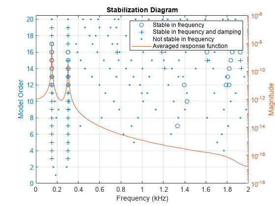

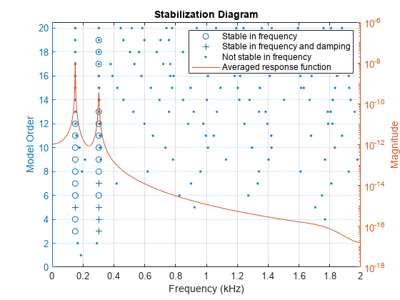
Repeat the computation, but now tighten the criteria for stability. Classify a given pole as stable in frequency if its natural frequency changes by less than 0.01% as the model order increases. Classify a given pole as stable in damping if the damping ratio estimate changes by less than 0.2% as the model order increases.

modalsd(frf,f,fs,'MaxModes',20,'SCriteria',[1e-4 0.002])

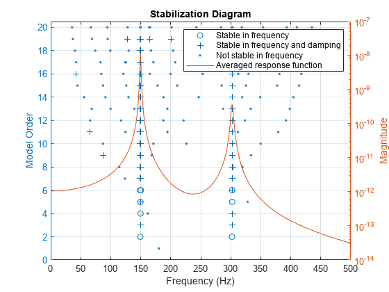
Restrict the frequency range to between 0 and 500 Hz. Relax the stability criteria to 0.5% for frequency and 10% for damping.

modalsd(frf,f,fs,'MaxModes',20,'SCriteria',[5e-3 0.1],'FreqRange',[0 500])

Repeat the computation using the least-squares rational function algorithm. Restrict the frequency range from 100 Hz to 350 Hz and identify up to 10 physical modes.

modalsd(frf,f,fs,'MaxModes',10,'FreqRange',[100 350],'FitMethod','lsrf')