Field-Oriented Control of Permanent Magnet Synchronous Machine
This example shows the basic workflow and key APIs for generating C code from a motor control algorithm, and for verifying its compiled behavior and execution time. Use processor-in-the-loop (PIL) simulation to gain confidence that the C code performs as expected when you integrate it with embedded software that interfaces with the motor hardware. Although the workflow uses a motor control application for a specific processor, you can apply the workflow to another application or processor.
The example uses a Field-Oriented Control algorithm for a Permanent Magnet Synchronous Machine. The control technique is common in motordrive systems for hybrid electric vehicles, manufacturing machinery, and industrial automation.
Overview
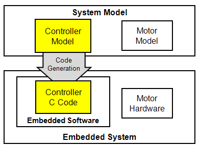
In this example, generate and verify C code from a control algorithm model, which you can integrate with additional embedded software required to interface to motor hardware.
Use a simulation environment to model and verify the behavior of a closed-loop motor control system. Once the control system behavior is within specification, generate C code from the controller model. After inspecting the code, assess its functional behavior and execution time by using processor-in-the-loop (PIL) testing.
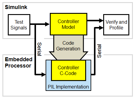
To facilitate PIL testing, select test signals to exercise the controller model and establish reference outputs. Review an example PIL implementation for a Texas Instruments™ F28335 processor that communicates with Simulink® on your development computer via a serial connection. You can use this example as a starting point to create a PIL implementation for your own processor. To measure execution time and verify execution behavior of the code on the embedded processor against the simulation reference outputs, run the controller model in PIL mode.
In the final implementation on the embedded processor, you integrate the generated controller C code with additional embedded software, such as peripherals and interrupts, required to interface with the motor hardware.
Notes
Simscape™ Electrical™ is required for system simulation in the section "Verify Behavior through System Simulation." It is not required for other tasks.
The Texas Instruments F28335 PIL implementation is a reference approach that you can apply to other processors. However, if you want to use this implementation directly, you need additional support files, compilers, and tools from Texas Instruments. For more information, see "Create PIL Implementation and Register with Simulink" in this example. The reference PIL implementation does not require the Texas Instruments C2000™ Embedded Target feature of Embedded Coder®, but C2000 users are encouraged to install Texas Instruments C2000 Support Package using Add-On Explorer.
Verify Behavior Through System Simulation
In this section, verify the controller in a closed loop system simulation.
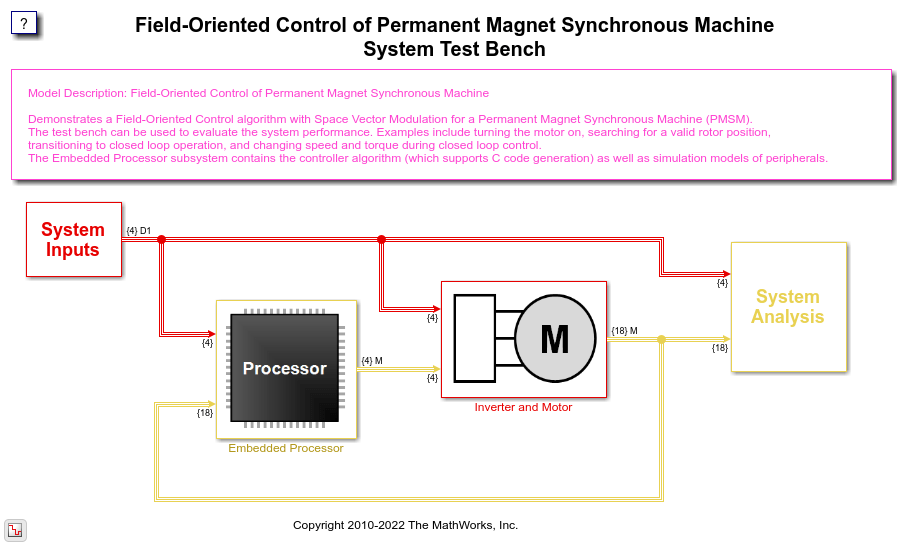
The system model test bench consists of test inputs, the embedded processor, the power electronics and motor hardware, and visualizations. You can use the system model to exercise the controller and explore its expected behavior. You can use the following commands to execute the model and plot logged signals.
open_system('PMSMSystem');
out_system = sim('PMSMSystem');
pmsmfoc_plotsignals(out_system.logsout);
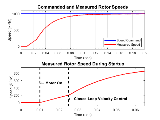
The plots show that the motor is stationary until the motor_on signal is true. The motor then spins in an open loop until a known position is detected, which is indicated by the encoder index pulse. The controller then transitions to closed loop operation and the motor reaches a steady state speed.
Explore Model Architecture
In this section, explore the model architecture including how data is specified, how the controller is partitioned from the test bench, and how controller is scheduled. This architecture facilitates system simulation, algorithmic code generation, and PIL testing.
A data definition file creates the MATLAB® data required for simulation and code generation. The PreLoadFcn callback of the system test bench model automatically runs the data definition file.
edit('pmsmfoc_data.m')
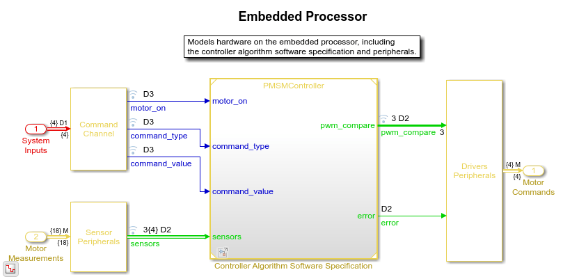
Within the system test bench model, the embedded processor is modeled as a combination of the peripherals and the controller software.
open_system('PMSMSystem/Embedded Processor');
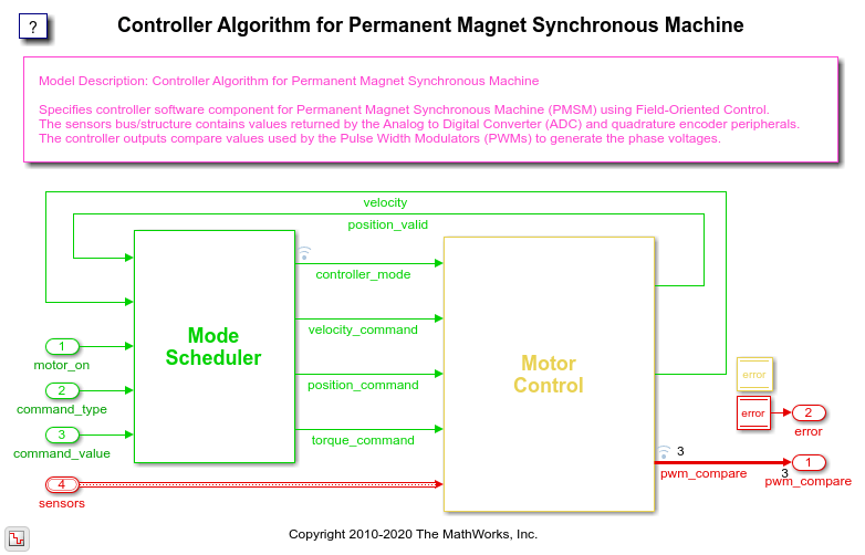
The controller software is specified in a separate model. Within this model, the Mode_Scheduler subsystem uses Stateflow® to schedule different modes of operation of the Motor_Control algorithm.
open_system('PMSMController');
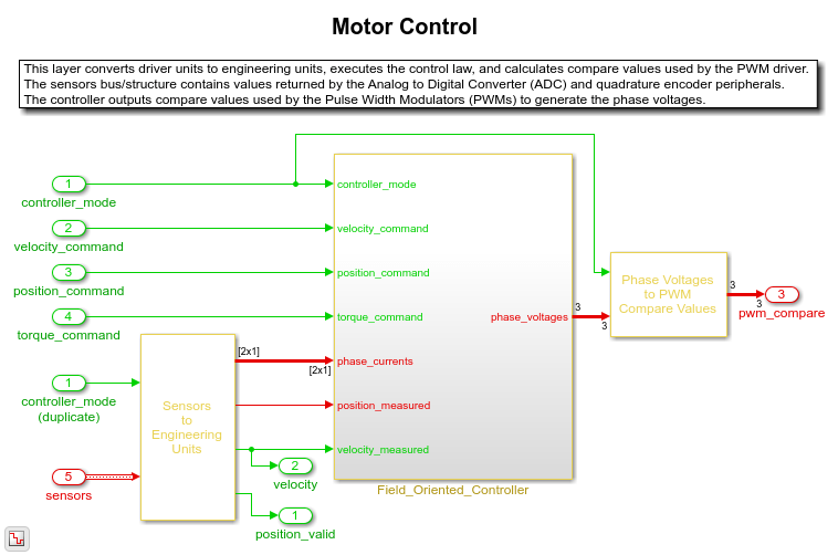
Within the Motor_Control subsystem, sensor signals are converted to engineering units and passed to the core controller algorithm. The controller algorithm calculates voltages. The voltages are then converted to a driver signal.
open_system('PMSMController/Motor_Control');
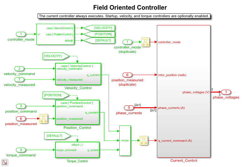
The primary control law is a field-oriented controller. The controller has a low rate outer loop that controls the speed, and a higher rate inner loop that controls the current.
open_system('PMSMController/Motor_Control/Field_Oriented_Controller');
The Velocity Controller outer loop is executed as a multiple of the Current Control loop time. You can view the MATLAB variables, which specify these sample times:
fprintf('High rate sample time = %f seconds\n', ctrlConst.TsHi)
fprintf('Low rate sample time  = %f seconds\n', ctrlConst.TsLo)
High rate sample time = 0.000040 seconds
Low rate sample time  = 0.005000 seconds
Notice that the highest rate in the controller algorithm is 25 kHz.
fprintf('High rate frequency = %5.0f Hz\n', 1/ctrlConst.TsHi)
High rate frequency = 25000 Hz
Generate Controller C Code for Integration into Embedded Application
In this section, generate and visually inspect the C code function for the controller.
To ease integration, the controller model is configured in single-tasking mode so that the generated code can be invoked using one function call. This function handles the lower and higher rates. The generated controller function must be executed at the high rate sample time.
The function prototype is specified in the model configuration parameters and the input and output ports are passed as arguments. You can view the function specification for the controller algorithm.
mdlFcn = RTW.getFunctionSpecification('PMSMController');
disp(mdlFcn.getPreview('init'))
disp(mdlFcn.getPreview('step'))
Controller_Init ( )
error = Controller ( motor_on, command_type, current_request, * sensors, * pwm_compare )
Through use of a global structure in the generated code, you can access the field-oriented controller proportional and integral gains. The global structure is specified in the data definition file.
disp(ctrlParams.Value)
disp(ctrlParams.CoderInfo)
                            Current_P: 10
                            Current_I: 10000
                           Velocity_P: 0.0050
                           Velocity_I: 0.0150
                           Position_P: 0.1000
                           Position_I: 0.6000
                  StartupAcceleration: 1
                       StartupCurrent: 0.2000
                   RampToStopVelocity: 20
             AdcZeroOffsetDriverUnits: 2.2522e+03
                 AdcDriverUnitsToAmps: 0.0049
    EncoderToMechanicalZeroOffsetRads: 0
                        PmsmPolePairs: 4

Simulink.CoderInfo
    StorageClass: 'ExportedGlobal'
      Identifier: ''
       Alignment: -1
Generate C code from the model.
slbuild('PMSMController');
### Starting build procedure for: PMSMController
### Successful completion of build procedure for: PMSMController

Build Summary

Top model targets built:

Model           Action                        Rebuild Reason
================================================================================================
PMSMController  Code generated and compiled.  Code generation information file does not exist.

1 of 1 models built (0 models already up to date)
Build duration: 0h 0m 29.573s
Use the generated report to inspect the generated C code file and verify that the correct step and initialization functions are generated. Also verify that the parameter structure is created as a global variable.
Specify Reference Behavior for Controller Model
In this section, specify test inputs and a reference output to help verify behavior and profile execution time during PIL testing.
Make a local copy of the controller model and load a set of test input signals that exercise the different modes within the controller. Configure the controller model to attach the logged signals to input ports. Then execute the controller model and log the output port signal to the workspace.
Configuration parameters of the controller model that specify the reference behavior and test environment change as described below. Blocks and parameters that specify the controller model's design and generate production code do not change. However, to avoid modifying any part of the installed controller model, save the model and change its name to PMSMControllerLocal.slx.
save_system('PMSMController','PMSMControllerLocal.slx')
close_system('PMSMSystem',0);
close_system('PMSMController',0);

To profile execution times, select a set of test inputs that execute the paths of interest within the controller. One way to acquire these test inputs and reference output is to log them from the system simulation model.
in.motor_on      = out_system.logsout.getElement('motor_on').Values;
in.command_type  = out_system.logsout.getElement('command_type').Values;
in.command_value = out_system.logsout.getElement('command_value').Values;
in.sensors       = out_system.logsout.getElement('sensors').Values;
disp(in)
         motor_on: [1×1 timeseries]
     command_type: [1×1 timeseries]
    command_value: [1×1 timeseries]
          sensors: [1×1 struct]
You can attach signals to the input ports and import the signals into the controller model such that it can execute directly and independently in the system model. An advantage of this approach is that you can test and verify the controller model as a standalone component, facilitating reuse and integration with other system models or closed-loop test benches. To elaborate, or prepare, the controller model for testing, change its configuration parameters to attach input signals and log signals in the MATLAB workspace. You can make the changes through the Configuration Parameters dialog box, or programmatically as shown here.
set_param('PMSMControllerLocal',...
    'LoadExternalInput', 'on',...
    'ExternalInput', 'in.motor_on, in.command_type, in.command_value, in.sensors',...
    'StopTime','0.06',...
    'ZeroInternalMemoryAtStartup','on',...
    'SimulationMode', 'normal')
save_system('PMSMControllerLocal.slx')
You can now execute the controller model and plot the signal associated with the PWM Compare output port.
out = sim('PMSMControllerLocal');
controller_mode = out.logsout.getElement('controller_mode').Values;
pwm_compare_ref = out.logsout.getElement('pwm_compare').Values;
pmsmfoc_plotpwmcompare(controller_mode, pwm_compare_ref)
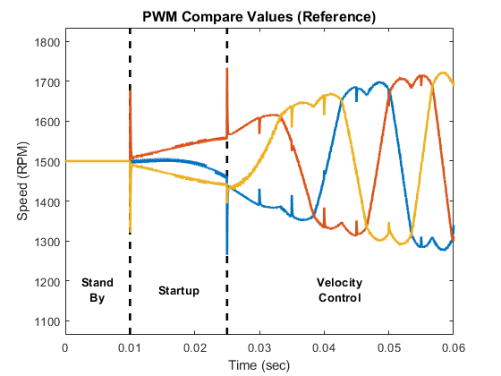
The logged output is used as the reference behavior for PIL testing.
Notice that the plot is annotated with information about the mode of the controller at each time step. This mode information is useful when interpreting execution profiling information.
Create PIL Implementation
In this section, study and use an example PIL implementation. Begin by reviewing prerequisite help documentation from Embedded Coder. Then copy the example PIL implementation into your local folder and register the implementation with Simulink. Review the approach used to develop the PIL implementation and explore the associated files to gain additional insight. If you are using a Spectrum Digital Inc. eZdsp F28335 board with Code Composer v4 and a serial connection, you can configure the PIL implementation to work with the controller model. If you are using a different processor, you can use the PIL implementation as a starting point for your implementation.
The fundamentals of creating a custom PIL implementation are described in Create PIL Target Connectivity Configuration for Simulink . Familiarize yourself with the concept of using the rtiostream API to facilitate communication between Simulink (host-side) and the embedded processor (target-side) during PIL testing. Note that Embedded Coder provides host-side drivers for the default TCP/IP implementation (for all platforms supported by Simulink) as well as a Windows® only version for serial communication. Build the generated code by using a makefile. See Customize Template Makefiles. To create a PIL implementation, you must perform several tasks in the embedded environment, including writing a target-side communications driver, writing a makefile to build the generated code, and automating download and execution of the built executable file.
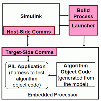
A PIL implementation, created by using the approach, is available for a Spectrum Digital Inc. eZdsp F28335 board. The implementation contains these target connectivity API components:
Host-Side Communication - The host-side connectivity driver is configured to use serial communication.
Target-Side Communication - The target-side communication is achieved using a handwritten serial implementation of the rtiostream functions as well as timer access functions.
Build Process - A makefile based approach is used to build the executable application.
Launcher - Downloading and running the executable is accomplished using the Debug Server Scripting (DSS) utility of Code Composer Studio™ v4 (CCSv4).
The PIL implementation was iteratively developed in three stages. You can use a similar approach when developing your PIL implementation.
Stage 1: Create serial communication application with CCSv4
Install CCSv4 and verify that it can connect with the F28335 eZdsp board.
Write an embedded application that sends and receives serial data.
Test the serial communication between your development computer and the embedded application.
Identify the commands and options for the compiler, linker, and archiver to build the application using a makefile.
Download and run the application from a Windows Command Prompt using the DSS utility.
Stage 2: Implement and test embedded serial rtiostream and launch automation with MATLAB
Extend the serial application to implement the rtiostream API functions for echoing data. Write the rtIOStreamOpen to perform general board initialization, including configuring the serial port.
Verify sending and receiving serial data with the embedded processor from MATLAB using the rtiostream_wrapper function.
Download and run the application from MATLAB using the system command to call the DSS utility.
Stage 3: Implement and test connectivity configuration with Simulink
Create a connectivity configuration class to configure the host-side serial communication, specify which target-side code files from the rtiostream application must be included in the build process, specify how to access a timer that is used to collect profiling data, and integrate calling the DSS utility to launch the embedded application.
Create a tool specification makefile (
target_tools.mk) which specifies the commands and options for the compiler, linker, and archiver. This makefile is included by the template makefile (target_tools.mk).Create a template makefile (
ec_target.tmf) that includestarget_tools.mk.Identify parameters which might be installation dependent and store them as MATLAB preferences.
Create a Simulink customization file that specifies when the PIL implementation is valid.
The files associated with the PIL implementation are included with Embedded Coder, but are not on the MATLAB path. To explore the files, you can copy them into a local folder. You can register the PIL implementation by adding the folder to the MATLAB path and refreshing the Simulink customizations.
addpath(genpath(fullfile('.','examplePilF28335')))
sl_refresh_customizations
Use MATLAB preferences to specify path information and the host serial COM port number. If you are using the PIL implementation directly, you must specify these preferences as appropriate for your configuration.
setpref('examplePilF28335','examplePilF28335Dir', fullfile('.','examplePilF28335'));
setpref('examplePilF28335','CCSRootDir',          'C:\Program Files\Texas Instruments\ccsv4');
setpref('examplePilF28335','TI_F28xxx_SysSWDir',  'C:\Program Files\Texas Instruments\TI_F28xxx_SysSW');
setpref('examplePilF28335','targetConfigFile',    fullfile('.','examplePilF28335','f28335_ezdsp.ccxml'));
setpref('examplePilF28335','baudRate',            115200);
setpref('examplePilF28335','cpuClockRateMHz',     150);
setpref('examplePilF28335','boardConfigPLL',      10);
setpref('examplePilF28335','COMPort',             'COM4');
Note that the TI_F28xxx_SysSWDir preference points to a folder provided by Texas Instruments in their C2000 Experimenter Kit Application Software (sprc675.zip). These files are not included with Embedded Coder.
The PIL implementation is now ready to be used.
Prepare Controller Model for PIL Testing
Review the customization file used to register the PIL implementation, set the configuration parameters of the model to use the PIL implementation, and enable logging of controller outputs and execution profiling data.
When you start a PIL simulation, Simulink checks if a registered PIL implementation is valid. A customization file specifies which configuration parameters correspond to a valid PIL implementation. You can explore the customization file for the implementation by invoking the following command.
edit(fullfile('.','examplePilF28335','sl_customization.m'));
Note that the file specifies settings for the hardware device and the template makefile that are required for the use of the PIL implementation. You can modify the configuration parameters in the controller model to match the settings. You can make the modifications through the Configuration Parameters dialog box, or programmatically as shown here.
set_param('PMSMControllerLocal',...
       'ProdHWDeviceType', 'Texas Instruments->C2000',...
       'TemplateMakefile', 'ec_target.tmf',...
       'GenCodeOnly', 'off',...
       'SimulationMode', 'processor-in-the-loop (pil)')
For the PIL simulation, enable code execution profiling, logging execution-time metrics in the variable executionProfile.
set_param('PMSMControllerLocal',...
    'CodeExecutionProfiling', 'on',...
    'CodeExecutionProfileVariable','executionProfile',...
    'CodeProfilingSaveOptions','AllData');
save_system('PMSMControllerLocal.slx')
You can now run PIL simulations of the controller model.
Test Behavior and Execution Time of Generated Code
In this section run the controller model in PIL mode and explore the behavioral and execution profiling results. Verify that the behavior of the compiled controller code matches the reference simulation behavior, and then verify that the execution of the code meets timing requirements.
You can run the model and plot the PIL simulation results. When you run the model for the first time, Embedded Coder generates code for the algorithm, links the algorithm code with the serial communication interface code, builds the embedded application, downloads the application to the board, and begins the on-target simulation. Note that during subsequent PIL simulations, code is regenerated only if you change the model. Due to the overhead associated with the serial communication interface, the PIL simulation might run slower than the normal mode simulation.
The MATLAB commands below are intentionally commented out as they require connection to hardware and use of embedded development tools described previously. If you have the hardware connected and embedded development tools installed, uncomment and execute these lines to run the model, plot the results, and verify the behavior is numerically equivalent to the normal mode simulation. Otherwise, continue reviewing this section to learn about PIL execution analysis options.
% UNCOMMENT THE BELOW LINES TO RUN THE SIMULATION AND PLOT THE RESULTS
% if exist('slprj','dir'), rmdir('slprj','s'); end
% out = sim('PMSMControllerLocal')
% pwm_compare_pil = out.logsout.getElement('pwm_compare').Values;
% pmsmfoc_plotpwmcompare_pil(controller_mode, pwm_compare_pil, executionProfile)
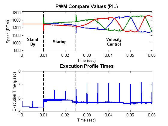
The upper plot is the output of the controller, PWM Compare. Note that the PIL simulation outputs look the same as the normal mode simulation outputs shown in the section "Establish Reference Behavior for Controller Model". To check numeric equivalence, you can subtract the normal mode simulation outputs from the PIL simulation outputs:
% UNCOMMENT THE BELOW LINE TO VERIFY NUMERIC EQUIVALENCE OF THE OUTPUTS
% pilErrorWithRespectToReference = sum(abs(pwm_compare_pil.Data - pwm_compare_pil.Data))
pilErrorWithRespectToReference =
0 0 0
The lower plot is the amount of time spent executing the controller model at each simulation time step. The "Stand By" state requires the least time. Small periodic spikes in execution time occur because the controller is multi-rate and single tasking. The periodic spikes correspond to the time required to run both the base rate and 5 millisecond rate code in the same task.
Since the controller must be executed at 25 kHz on the embedded processor, the algorithm must complete its execution within 40 microseconds (minus additional headroom requirements by other code, which may also be executing on the final application.) The profiling results indicate that the algorithm will execute within the time allotted for this configuration of the embedded environment.
The generated code is now verified to provide numerically equivalent results and meets the execution timing requirements for the test case.
close_system('PMSMControllerLocal',0);
close_system('power_utile',0);
The MATLAB preferences used in this PIL implementation are persistent between MATLAB sessions. If you want to remove the preferences, run these commands:
rmpref('examplePilF28335');
rmexamplePilF28335hooks();
Conclusion
Using a Field-Oriented Control algorithm for a Permanent Magnet Synchronous Machine, the example shows how you can use system-level simulation and algorithmic code generation to explore functional behavior of the controller algorithm. The example also shows a general approach for target integration, functional testing, and execution profiling for embedded processors. Once the algorithm is behaviorally correct, you can generate code from the controller model and test and profile the code on the target processor. For further testing, you can integrate the verified algorithm code with embedded software that interfaces with the motor hardware.
Related Topics
- SIL and PIL Simulations
- Choose a SIL or PIL Approach
- Create PIL Target Connectivity Configuration for Simulink
- Configure and Run SIL Simulation
- Create Execution-Time Profile for Generated Code
- MATLAB Project for FOC of PMSM with Quadrature Encoder (Motor Control Blockset)
- Algorithm-Export Workflows for Custom Hardware (Motor Control Blockset)
You can also select a web site from the following list:
Americas
- América Latina (Español)
- Canada (English)
- United States (English)
Europe
- Belgium (English)
- Denmark (English)
- Deutschland (Deutsch)
- España (Español)
- Finland (English)
- France (Français)
- Ireland (English)
- Italia (Italiano)
- Luxembourg (English)
- Netherlands (English)
- Norway (English)
- Österreich (Deutsch)
- Portugal (English)
- Sweden (English)
- Switzerland
- United Kingdom (English)