Frequency Domain Identification: Estimating Models Using Frequency Domain Data
This example shows how to estimate models using frequency domain data. The estimation and validation of models using frequency domain data work the same way as they do with time domain data. This provides a great amount of flexibility in estimation and analysis of models using time and frequency domain as well as spectral (FRF) data. You may simultaneously estimate models using data in both domains, compare and combine these models. A model estimated using time domain data may be validated using spectral data or vice-versa.
Frequency domain data cannot be used for estimation or validation of nonlinear models.
Introduction
Frequency domain experimental data are common in many applications. It could be that the data was collected as frequency response data (frequency functions: FRF) from the process using a frequency analyzer. It could also be that it is more practical to work with the input's and output's Fourier transforms (FFT of time-domain data), for example to handle periodic or band-limited data. (A band-limited continuous time signal has no frequency components above the Nyquist frequency). In System Identification Toolbox, frequency domain I/O data are represented the same way as time-domain data, i.e., using iddata objects. The 'Domain' property of the object must be set to 'Frequency'. Frequency response data are represented as complex vectors or as magnitude/phase vectors as a function of frequency. IDFRD objects in the toolbox are used to encapsulate FRFs, where a user specifies the complex response data and a frequency vector. Such IDDATA or IDFRD objects (and also FRD objects of Control System Toolbox) may be used seamlessly with any estimation routine (such as procest, tfest etc).
Inspecting Frequency Domain Data
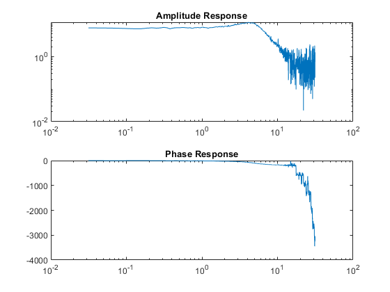
Let us begin by loading some frequency domain data:
load demofr
This MAT-file contains frequency response data at frequencies W, with the amplitude response AMP and the phase response PHA. Let us first have a look at the data:
subplot(211), loglog(W,AMP),title('Amplitude Response')
subplot(212), semilogx(W,PHA),title('Phase Response')
This experimental data will now be stored as an IDFRD object. First transform amplitude and phase to a complex valued response:
zfr = AMP.*exp(1i*PHA*pi/180);
Ts = 0.1;
gfr = idfrd(zfr,W,Ts);
Ts is the sample time of the underlying data. If the data corresponds to continuous time, for example since the input has been band-limited, use Ts = 0.
Note: If you have the Control System Toolbox™, you could use an FRD object instead of the IDFRD object. IDFRD has options for more information, like disturbance spectra and uncertainty measures which are not available in FRD objects.
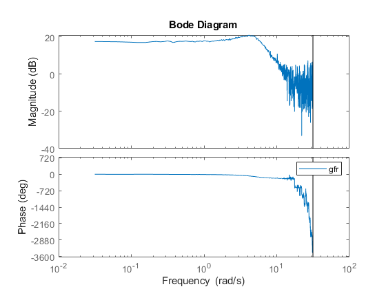
The IDFRD object gfr now contains the data, and it can be plotted and analyzed in different ways. To view the data, we may use plot or bode:
clf
bode(gfr), legend('gfr')
Estimating Models Using Frequency Response (FRF) Data
To estimate models, you can now use gfr as a data set with all the commands of the toolbox in a transparent fashion. The only restriction is that noise models cannot be built. This means that for polynomial models only OE (output-error models) apply, and for state-space models, you have to fix K = 0.
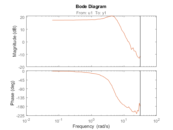
m1 = oe(gfr,[2 2 1]) % Discrete-time Output error (transfer function) model
ms = ssest(gfr) % Continuous-time state-space model with default choice of order
mproc = procest(gfr,'P2UDZ') % 2nd-order, continuous-time model with underdamped poles
compare(gfr,m1,ms,mproc)
L = findobj(gcf,'type','legend');
L.Location = 'southwest'; % move legend to non-overlapping location
m1 =
Discrete-time OE model: y(t) = [B(z)/F(z)]u(t) + e(t)
  B(z) = 0.9986 z^-1 + 0.4968 z^-2

  F(z) = 1 - 1.499 z^-1 + 0.6998 z^-2

Sample time: 0.1 seconds

Parameterization:
   Polynomial orders:   nb=2   nf=2   nk=1
   Number of free coefficients: 4
   Use "polydata", "getpvec", "getcov" for parameters and their uncertainties.

Status:
Estimated using OE on frequency response data "gfr".
Fit to estimation data: 88.04%
FPE: 0.2512, MSE: 0.2492


ms =
  Continuous-time identified state-space model:
      dx/dt = A x(t) + B u(t) + K e(t)
       y(t) = C x(t) + D u(t) + e(t)

  A =
           x1      x2
   x1  -1.785   3.097
   x2  -6.835  -1.785

  B =
          u1
   x1  -4.15
   x2  27.17

  C =
           x1      x2
   y1    1.97  0.3947

  D =
       u1
   y1   0

  K =
       y1
   x1   0
   x2   0

Parameterization:
   FREE form (all coefficients in A, B, C free).
   Feedthrough: none
   Disturbance component: none
   Number of free coefficients: 8
   Use "idssdata", "getpvec", "getcov" for parameters and their uncertainties.

Status:
Estimated using SSEST on frequency response data "gfr".
Fit to estimation data: 88.04%
FPE: 0.2512, MSE: 0.2492


mproc =

Process model with transfer function:
                     1+Tz*s
  G(s) = Kp * ---------------------- * exp(-Td*s)
              1+2*Zeta*Tw*s+(Tw*s)^2

         Kp = 7.4523
         Tw = 0.20266
       Zeta = 0.36165
         Td = 0
         Tz = 0.01407

Parameterization:
    {'P2DUZ'}
   Number of free coefficients: 5
   Use "getpvec", "getcov" for parameters and their uncertainties.

Status:
Estimated using PROCEST on frequency response data "gfr".
Fit to estimation data: 88.04%
FPE: 0.2517, MSE: 0.2492
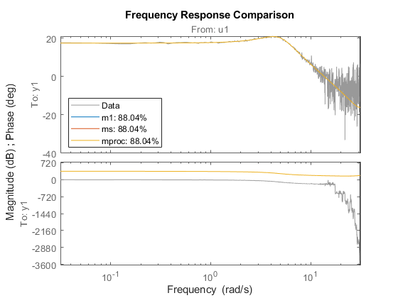
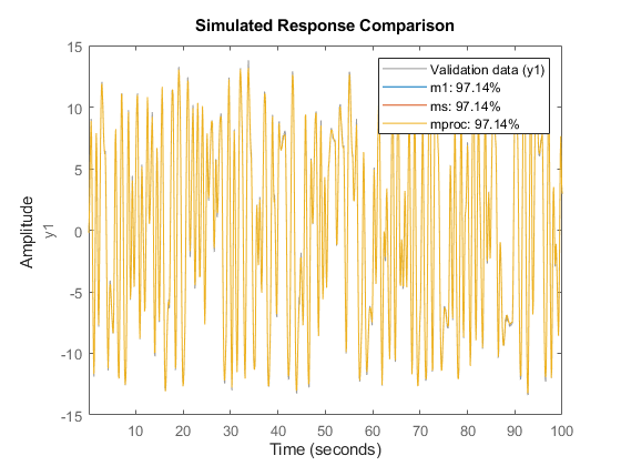
As shown above a variety of linear model types may be estimated in both continuous and discrete time domains, using spectral data. These models may be validated using, time-domain data. The time-domain I/O data set ztime, for example, is collected from the same system, and can be used for validation of m1, ms and mproc:
compare(ztime,m1,ms,mproc) %validation in a different domain
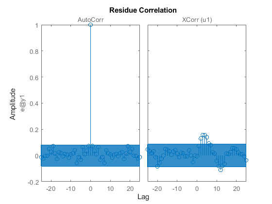
We may also look at the residuals to affirm the quality of the model using the validation data ztime. As observed, the residuals are almost white:
resid(ztime,mproc) % Residuals plot
Condensing Data Using SPAFDR
An important reason to work with frequency response data is that it is easy to condense the information with little loss. The command SPAFDR allows you to compute smoothed response data over limited frequencies, for example with logarithmic spacing. Here is an example where the gfr data is condensed to 100 logarithmically spaced frequency values. With a similar technique, also the original time domain data can be condensed:
sgfr = spafdr(gfr) % spectral estimation with frequency-dependent resolution
sz = spafdr(ztime); % spectral estimation using time-domain data
clf
bode(gfr,sgfr,sz)
axis([pi/100 10*pi, -272 105])
legend('gfr (raw data)','sgfr','sz','location','southwest')
sgfr =
IDFRD model.
Contains Frequency Response Data for 1 output(s) and 1 input(s), and the spectra for disturbances at the outputs.
Response data and disturbance spectra are available at 100 frequency points, ranging from 0.03142 rad/s to 31.42 rad/s.

Sample time: 0.1 seconds
Output channels: 'y1'
Input channels: 'u1'
Status:
Estimated using SPAFDR on frequency response data "gfr".
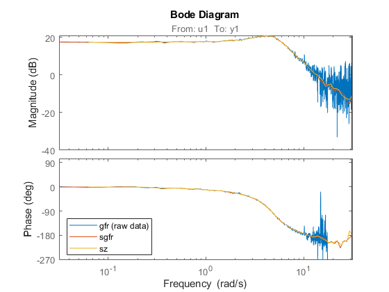
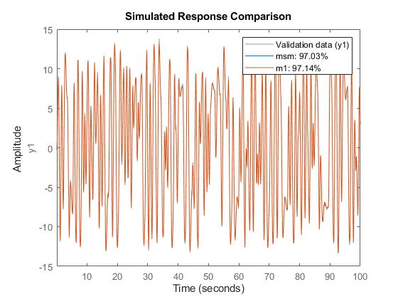
The Bode plots show that the information in the smoothed data has been taken well care of. Now, these data records with 100 points can very well be used for model estimation. For example:
msm = oe(sgfr,[2 2 1]);
compare(ztime,msm,m1) % msm has the same accuracy as M1 (based on 1000 points)
Estimation Using Frequency-Domain I/O Data
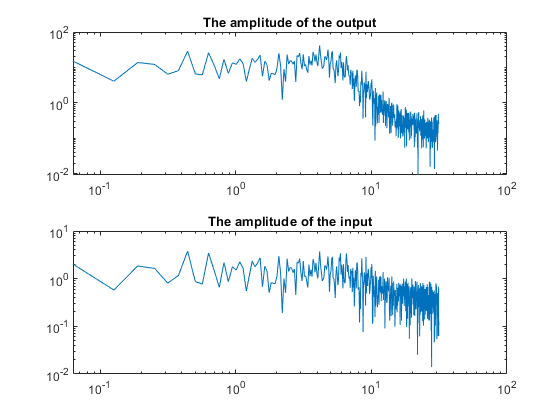
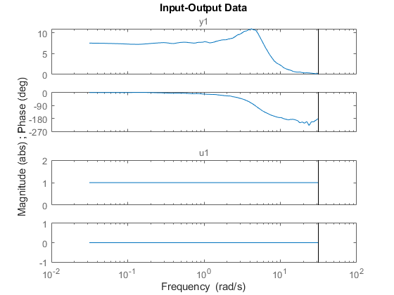
It may be that the measurements are available as Fourier transforms of inputs and output. Such frequency domain data from the system are given as the signals Y and U. In loglog plots they look like
Wfd = (0:500)'*10*pi/500;
subplot(211),loglog(Wfd,abs(Y)),title('The amplitude of the output')
subplot(212),loglog(Wfd,abs(U)),title('The amplitude of the input')
The frequency response data is essentially the ratio between Y and U. To collect the frequency domain data as an IDDATA object, do as follows:
ZFD = iddata(Y, U, 'Ts', 0.1, 'Frequency', Wfd)
ZFD =

Frequency domain data set with responses at 501 frequencies.
Frequency range: 0 to 31.416 rad/seconds
Sample time: 0.1 seconds

Outputs      Unit (if specified)
   y1

Inputs       Unit (if specified)
   u1
Now, again the frequency domain data set ZFD can be used as data in all estimation routines, just as time domain data and frequency response data:
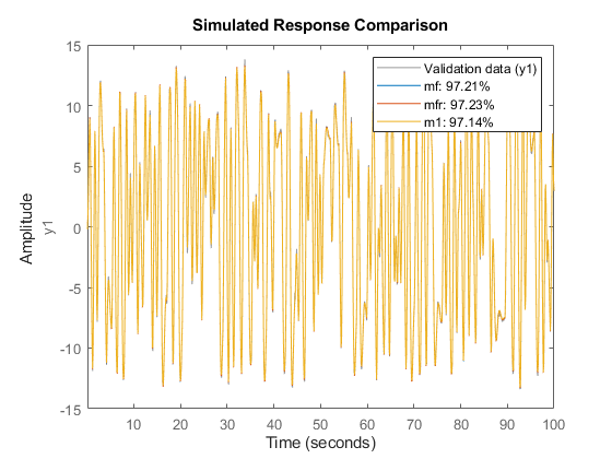
mf = ssest(ZFD)   % SSEST picks best order in 1:10 range when called this way
mfr = ssregest(ZFD) % an alternative regularized reduction based state-space estimator
clf
compare(ztime,mf,mfr,m1)
mf =
  Continuous-time identified state-space model:
      dx/dt = A x(t) + B u(t) + K e(t)
       y(t) = C x(t) + D u(t) + e(t)

  A =
           x1      x2
   x1   -1.78   3.095
   x2  -6.812   -1.78

  B =
          u1
   x1   1.32
   x2  28.61

  C =
              x1         x2
   y1          2  6.416e-08

  D =
       u1
   y1   0

  K =
       y1
   x1   0
   x2   0

Parameterization:
   FREE form (all coefficients in A, B, C free).
   Feedthrough: none
   Disturbance component: none
   Number of free coefficients: 8
   Use "idssdata", "getpvec", "getcov" for parameters and their uncertainties.

Status:
Estimated using SSEST on frequency domain data "ZFD".
Fit to estimation data: 97.21%
FPE: 0.04288, MSE: 0.04186


mfr =
  Discrete-time identified state-space model:
    x(t+Ts) = A x(t) + B u(t) + K e(t)
       y(t) = C x(t) + D u(t) + e(t)

  A =
                x1          x2          x3          x4          x5          x6
   x1        0.701    -0.05307     -0.4345   -0.006642    -0.08085     -0.1158
   x2      -0.4539    -0.09623     -0.3629      0.2113     -0.2219      0.3536
   x3       0.1719     -0.3996      0.4385    -0.01558      0.1768      0.2467
   x4      -0.1821      0.3465      0.3292     -0.1357     -0.2578      0.2483
   x5     -0.09939      -0.338      0.1236     -0.2537      -0.387     0.05591
   x6     -0.06004       0.226     0.04117     -0.6891     -0.0873      0.2818
   x7       0.1056     -0.1859    -0.04223       0.629     -0.1968      0.7077
   x8      0.05337      0.1948     0.06355    -0.09052      0.4216      0.3997
   x9      0.01696     0.05961     0.04891     0.01251     0.03521      0.3876
   x10    -0.01727     -0.1232    -0.03586      0.1187     -0.1738    -0.05051

                x7          x8          x9         x10
   x1       0.3087    0.007547    -0.02011     -0.1469
   x2      0.01728    -0.04967     -0.1144     0.03883
   x3     -0.07107     -0.2977       0.129    -0.06179
   x4     -0.08461     0.03541     0.06711     -0.1759
   x5       0.5324      0.1778      0.1114  -2.119e-05
   x6       -0.155     -0.5047      -0.285      0.3976
   x7      -0.2406     -0.5628    -0.09159      0.4845
   x8       0.5674     -0.3337      -0.105      0.1995
   x9      -0.2024      0.4718    -0.01861      0.5838
   x10    -0.01243      0.2968     -0.6808     -0.7726

  B =
              u1
   x1   -0.09482
   x2     0.7665
   x3     -1.036
   x4      0.162
   x5    -0.2926
   x6     0.0805
   x7     0.1277
   x8   -0.02441
   x9    -0.0288
   x10   0.03776

  C =
            x1       x2       x3       x4       x5       x6       x7
   y1    1.956  -0.4539   -1.805   -1.356   0.3662    1.691  -0.8489

            x8       x9      x10
   y1    0.148   0.5203  -0.4013

  D =
       u1
   y1   0

  K =
               y1
   x1      0.1063
   x2   -0.007395
   x3      0.0426
   x4    0.004966
   x5    -0.01505
   x6   -0.005483
   x7   0.0004218
   x8   -0.001044
   x9   -0.003066
   x10   0.002273

Sample time: 0.1 seconds

Parameterization:
   FREE form (all coefficients in A, B, C free).
   Feedthrough: none
   Disturbance component: estimate
   Number of free coefficients: 130
   Use "idssdata", "getpvec", "getcov" for parameters and their uncertainties.

Status:
Estimated using SSREGEST on frequency domain data "ZFD".
Fit to estimation data: 76.61% (prediction focus)
FPE: 3.448, MSE: 2.938
Transformations Between Data Representations (Time - Frequency)
Time and frequency domain input-output data sets can be transformed to either domain by using FFT and IFFT. These commands are adapted to IDDATA objects:
dataf = fft(ztime)
datat = ifft(dataf)
dataf =

Frequency domain data set with responses at 501 frequencies.
Frequency range: 0 to 31.416 rad/seconds
Sample time: 0.1 seconds

Outputs      Unit (if specified)
   y1

Inputs       Unit (if specified)
   u1


datat =

Time domain data set with 1000 samples.
Sample time: 0.1 seconds

Outputs      Unit (if specified)
   y1

Inputs       Unit (if specified)
   u1
Time and frequency domain input-output data can be transformed to frequency response data by SPAFDR, SPA and ETFE:
g1 = spafdr(ztime)
g2 = spafdr(ZFD);
clf;
bode(g1,g2)
g1 =
IDFRD model.
Contains Frequency Response Data for 1 output(s) and 1 input(s), and the spectra for disturbances at the outputs.
Response data and disturbance spectra are available at 100 frequency points, ranging from 0.06283 rad/s to 31.42 rad/s.

Sample time: 0.1 seconds
Output channels: 'y1'
Input channels: 'u1'
Status:
Estimated using SPAFDR on time domain data "ztime".
Frequency response data can also be transformed to more smoothed data (less resolution and less data) by SPAFDR and SPA;
g3 = spafdr(gfr);
Frequency response data can be transformed to frequency domain input-output signals by the command IDDATA:
gfd = iddata(g3)
plot(gfd)
gfd =

Frequency domain data set with responses at 100 frequencies.
Frequency range: 0.031416 to 31.416 rad/seconds
Sample time: 0.1 seconds

Outputs      Unit (if specified)
   y1

Inputs       Unit (if specified)
   u1
Using Continuous-time Frequency-domain Data to Estimate Continuous-time Models
Time domain data can naturally only be stored and dealt with as discrete-time, sampled data. Frequency domain data have the advantage that continuous time data can be represented correctly. Suppose that the underlying continuous time signals have no frequency information above the Nyquist frequency, e.g. because they are sampled fast, or the input has no frequency component above the Nyquist frequency and that the data has been collected from a steady-state experiment. Then the Discrete Fourier transforms (DFT) of the data also are the Fourier transforms of the continuous time signals, at the chosen frequencies. They can therefore be used to directly fit continuous time models.
This will be illustrated by the following example.
Consider the continuous time system:
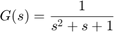
m0 = idpoly(1,1,1,1,[1 1 1],'ts',0)
m0 =
Continuous-time OE model: y(t) = [B(s)/F(s)]u(t) + e(t)
  B(s) = 1

  F(s) = s^2 + s + 1

Parameterization:
   Polynomial orders:   nb=1   nf=2   nk=0
   Number of free coefficients: 3
   Use "polydata", "getpvec", "getcov" for parameters and their uncertainties.

Status:
Created by direct construction or transformation. Not estimated.
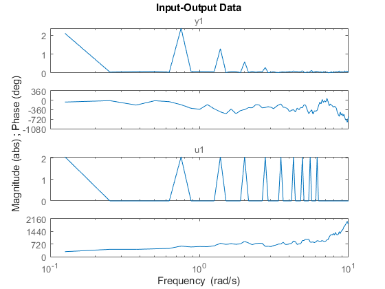
Load data that comes from steady-state simulation of this system using periodic inputs. The collected data was converted into frequency domain and saved in CTFDData.mat file.
load CTFDData.mat dataf % load continuous-time frequency-domain data.
Look at the data:
plot(dataf)
set(gca,'XLim',[0.1 10])
Using dataf for estimation will by default give continuous time models: State-space:
m4 = ssest(dataf,2); %Second order continuous-time model
For a polynomial model with nb = 2 numerator coefficient and nf = 2 estimated denominator coefficients use:
nb = 2;
nf = 2;
m5 = oe(dataf,[nb nf])
m5 =
Continuous-time OE model: y(t) = [B(s)/F(s)]u(t) + e(t)
  B(s) = -0.01814 s + 1.008

  F(s) = s^2 + 1.001 s + 0.9967

Parameterization:
   Polynomial orders:   nb=2   nf=2   nk=0
   Number of free coefficients: 4
   Use "polydata", "getpvec", "getcov" for parameters and their uncertainties.

Status:
Estimated using OE on frequency domain data "dataf".
Fit to estimation data: 70.15%
FPE: 0.00491, MSE: 0.00468
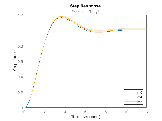
Compare step responses with uncertainty of the true system m0 and the models m4 and m5. The confidence intervals are shown with patches in the plot.
clf
h = stepplot(m0,m4,m5);
showConfidence(h,1)
legend('show','location','southeast')
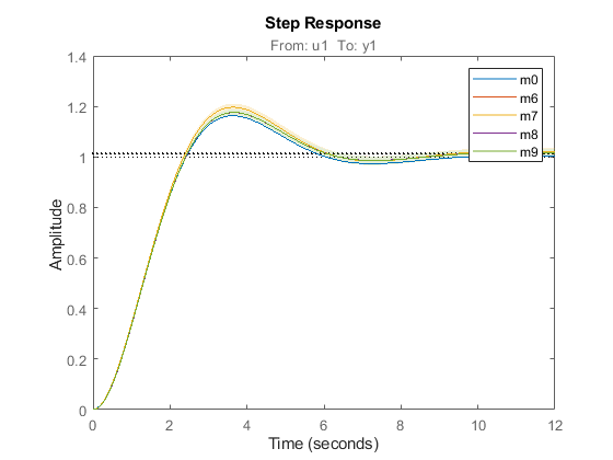
Although it was not necessary in this case, it is generally advised to focus the fit to a limited frequency band (low pass filter the data) when estimating using continuous time data. The system has a bandwidth of about 3 rad/s, and was excited by sinusoids up to 6.2 rad/s. A reasonable frequency range to focus the fit to is then [0 7] rad/s:
m6 = ssest(dataf,2,ssestOptions('WeightingFilter',[0 7])) % state space model
m6 =
  Continuous-time identified state-space model:
      dx/dt = A x(t) + B u(t) + K e(t)
       y(t) = C x(t) + D u(t) + e(t)

  A =
            x1       x2
   x1  -0.5011    1.001
   x2  -0.7446  -0.5011

  B =
             u1
   x1  -0.01706
   x2     1.016

  C =
               x1          x2
   y1       1.001  -0.0005347

  D =
       u1
   y1   0

  K =
       y1
   x1   0
   x2   0

Parameterization:
   FREE form (all coefficients in A, B, C free).
   Feedthrough: none
   Disturbance component: none
   Number of free coefficients: 8
   Use "idssdata", "getpvec", "getcov" for parameters and their uncertainties.

Status:
Estimated using SSEST on frequency domain data "dataf".
Fit to estimation data: 87.03% (data prefiltered)
FPE: 0.004832, MSE: 0.003631
m7 = oe(dataf,[1 2],oeOptions('WeightingFilter',[0 7])) % polynomial model of Output Error structure
m7 =
Continuous-time OE model: y(t) = [B(s)/F(s)]u(t) + e(t)
  B(s) = 0.9861

  F(s) = s^2 + 0.9498 s + 0.9704

Parameterization:
   Polynomial orders:   nb=1   nf=2   nk=0
   Number of free coefficients: 3
   Use "polydata", "getpvec", "getcov" for parameters and their uncertainties.

Status:
Estimated using OE on frequency domain data "dataf".
Fit to estimation data: 86.81% (data prefiltered)
FPE: 0.004902, MSE: 0.003752
opt = procestOptions('SearchMethod','lsqnonlin',...
   'WeightingFilter',[0 7]); % Requires Optimization Toolbox(TM)
m8 = procest(dataf,'P2UZ',opt)  % process model with underdamped poles
m8 =

Process model with transfer function:
                     1+Tz*s
  G(s) = Kp * ----------------------
              1+2*Zeta*Tw*s+(Tw*s)^2

         Kp = 1.0124
         Tw = 1.0019
       Zeta = 0.5021
         Tz = -0.017474

Parameterization:
    {'P2UZ'}
   Number of free coefficients: 4
   Use "getpvec", "getcov" for parameters and their uncertainties.

Status:
Estimated using PROCEST on frequency domain data "dataf".
Fit to estimation data: 87.03% (data prefiltered)
FPE: 0.004832, MSE: 0.003631
opt = tfestOptions('SearchMethod','lsqnonlin',...
   'WeightingFilter',[0 7]); % Requires Optimization Toolbox
m9 = tfest(dataf,2,opt) % transfer function with 2 poles
m9 =

  From input "u1" to output "y1":
  -0.01662 s + 1.007
  ------------------
   s^2 + s + 0.995

Continuous-time identified transfer function.

Parameterization:
   Number of poles: 2   Number of zeros: 1
   Number of free coefficients: 4
   Use "tfdata", "getpvec", "getcov" for parameters and their uncertainties.

Status:
Estimated using TFEST on frequency domain data "dataf".
Fit to estimation data: 87.03% (data prefiltered)
FPE: 0.00491, MSE: 0.003629
h = stepplot(m0,m6,m7,m8,m9);
showConfidence(h,1)
legend('show')
Conclusions
We saw how time, frequency and spectral data can seamlessly be used to estimate a variety of linear models in both continuous and discrete time domains. The models may be validated and compared in domains different from the ones they were estimated in. The data formats (time, frequency and spectrum) are interconvertible, using methods such as fft, ifft, spafdr and spa. Furthermore, direct, continuous-time estimation is achievable by using tfest, ssest and procest estimation routines. The seamless use of data in any domain for estimation and analysis is an important feature of System Identification Toolbox.
See Also
Related Topics
You can also select a web site from the following list:
Americas
- América Latina (Español)
- Canada (English)
- United States (English)
Europe
- Belgium (English)
- Denmark (English)
- Deutschland (Deutsch)
- España (Español)
- Finland (English)
- France (Français)
- Ireland (English)
- Italia (Italiano)
- Luxembourg (English)
- Netherlands (English)
- Norway (English)
- Österreich (Deutsch)
- Portugal (English)
- Sweden (English)
- Switzerland
- United Kingdom (English)