Classify Breast Tumors from Ultrasound Images Using Fuzzy Inference System

This example shows how to use fuzzy inference systems (FISs) to classify breast tumors as benign or malignant using radiomics features from ultrasound images. This example is adapted from Classify Breast Tumors from Ultrasound Images Using Radiomics Features (Medical Imaging Toolbox).

Radiomics extracts a large number of features from medical images related to the shape, intensity distribution, and texture of the specified region of interest (ROI). The extracted radiomics features contain useful information about the medical image that you can use in a classification application for automated diagnosis. This example extracts radiomics features from the tumor regions of breast ultrasound images and uses these features in a fuzzy inference system (FIS) tree to classify whether the tumor is benign or malignant.

Data Set

This example uses the Breast Ultrasound Images (BUSI) data set [1]. The BUSI data set contains 2-D ultrasound images stored in the PNG file format. The total size of the data set is 196 MB. The data set contains 133 normal scans that have no tumors, 437 scans with benign tumors, and 210 scans with malignant tumors. Each ultrasound image has a corresponding tumor mask image and a label of normal, benign, or malignant. The tumor mask labels have been reviewed by clinical radiologists [1]. The normal scans do not have any tumor regions in their corresponding tumor mask images. The example uses images from only the tumor groups.

Download the data set.

zipFile = matlab.internal.examples.downloadSupportFile("image","data/Dataset_BUSI.zip");
filepath = fileparts(zipFile);

Create a folder and unzip the dataset to that folder.

imageDir = fullfile(filepath,"Dataset_BUSI_with_GT");

if ~exist(imageDir,"dir")
    unzip(zipFile,filepath)
end

Load and Prepare Data

Prepare the data for training by performing the following tasks.

1. Label each image as normal, benign, or malignant, based on the name of its folder.

2. Separate the ultrasound and mask images.

3. Retain images from only the tumor groups.

4. Create a variable to store labels.

[tumorDS,maskDS,labels] = prepareTumorData(imageDir);

tumorDS and maskDS are image data stores containing the tumor and mask images, respectively. labels contains the tumor type of each data point.

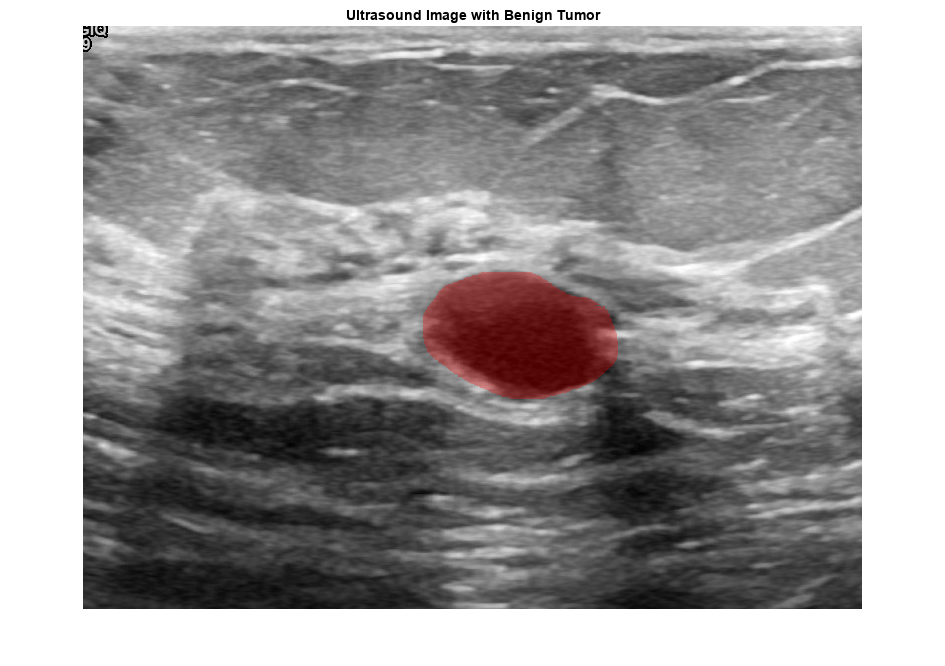
View Sample Data

View an ultrasound image that contains a benign tumor with the tumor mask on the image.

viewTumorImage(tumorDS,maskDS,146, ...
    "benign","Ultrasound Image with Benign Tumor")

View an ultrasound image that contains a malignant tumor with the tumor mask on the image.

viewTumorImage(tumorDS,maskDS,200, ...
    "malignant","Ultrasound Image with Malignant Tumor")

Create Training and Test Data Sets

Split the data into 70 percent training data and 30 percent test data using holdout validation. Use a default random number generator to reproduce the data partition.

n = length(labels);
p = 0.3;
rng("default")
datapartition = cvpartition(n,"Holdout",p);
idxTrain = training(datapartition);
idxTest = test(datapartition);

Create separate labels for the training and test data.

labelsTrain = labels(idxTrain);
labelsTest = labels(idxTest);

Create Radiomics Features for Training

Depending on your system configuration, the feature computation can take a long time. To use a precalculated set of radiomics features, set computeRadiomics to false.

computeRadiomics = false;

Compute radiomics features for training using the createRadiomicsFeatures helper function. For more information about creating these features, see Classify Breast Tumors from Ultrasound Images Using Radiomics Features (Medical Imaging Toolbox).

[trainInputFeatures,trainOutput,featureNames,selectedFeatures] = createRadiomicsFeatures( ...
    tumorDS,maskDS,"train",labelsTrain,idxTrain,computeRadiomics);

Visualize Radiomics Features

Compute the number of features after feature selection.

numFeatures = size(trainInputFeatures,2)

numFeatures = 12

Visualize each selected feature for the training data alongside their labels. The first bar in the visualization shows the ground truth classification of the training data, with benign tumors indicated in blue and malignant tumors indicated in yellow. The rest of the bars show each of the selected features. Although the colormap of each feature is different, the trend of each feature changes where the malignancy changes. For example, for the VolumeDensityConvexHull2D feature, the bottom portion of the bar corresponding to malignant tumors is more blue than the upper portion corresponding to benign tumors.

figure(Position=[0 0 1500 500])
layout = tiledlayout(1,numFeatures + 1);
layout.Title.String = "Radiomics Features of Training Data";
tile = nexttile;
imagesc(trainOutput)
set(tile,XTick=[],YTick=[])
ylabel("Malignancy",Interpreter="none")
for i = 1:numFeatures
    tile = nexttile;
    imagesc(trainInputFeatures(:,i))
    set(tile,XTick=[],YTick=[])
    ylabel(featureNames{i},Interpreter="none")
end

FIS Tree for Classification

Use the training data to create and train fuzzy systems for breast tumor classification.

This example uses multiple fuzzy systems in a FIS tree configuration to avoid the large rule base of a monolithic FIS having 12 input features. A large rule base is difficult to explain and often results in a lengthy training process, which might not converge to an expected solution. A human operator can generally explain a FIS having three to five inputs. This example uses a FIS tree with the following FISs having a maximum of 4 inputs:

• fis1 uses the VolumeMesh2D, SurfaceVolumeRatio2D, Compactness2_2D, and SphericalDisproportion2D features as inputs and produces an intermediate malignancy value, malignancy1.

• fis2 uses the CentreOfMassShift2D, MajorAxisLength2D, MinorAxisLength2D, and Elongation2D features as inputs and produces an intermediate malignancy value, malignancy2.

• fis3 uses the VolumeDensityAABB_2D, AreaDensityAEE_2D, VolumeDensityConvexHull2D, and IntegratedIntensity2D features as inputs and produces an intermediate malignancy value, malignancy3.

• fis4 uses the intermediate malignancy values as inputs to produce a combined malignancy value corresponding to a specific radiomics feature vector.

fis1, fis2, and fis3 use 2 membership functions (MFs) for each input and 5 MFs for each output, whereas, fis4 uses two MFs for each input and 4 MFs for the output.

For this example, the radiomics features are arbitrarily arranged into three input groups for fis1, fis2, and fis3. You can also rank and associate the features into different input groups using their correlation coefficient values or principal component analysis.

Calculate the minimum and maximum feature values to specify the input ranges of the fuzzy systems.

minMaxRanges = double([min(trainInputFeatures);max(trainInputFeatures)]);

Create the fuzzy systems.

fis1 = createFIS("fis1", minMaxRanges(:,1:4), ...
    featureNames(1:4),"malignancy1");
fis2 = createFIS("fis2",minMaxRanges(:,5:8), ...
    featureNames(5:8),"malignancy2");
fis3 = createFIS("fis3",minMaxRanges(:,9:12), ...
    featureNames(9:12),"malignancy3");
fis4 = createFIS("fis4",repmat([0;1],1,3), ...
    {"malignancy1","malignancy2","malignancy3"},"malignancy");
fis = [fis1 fis2 fis3 fis4];

Define the connections between the fuzzy systems.

connections = [...
    "fis1/malignancy1" "fis4/malignancy1"; ...
    "fis2/malignancy2" "fis4/malignancy2"; ...
    "fis3/malignancy3" "fis4/malignancy3" ...
    ];

Construct a FIS tree using the fuzzy systems and the connections.

fisT = fistree(fis,connections);

Visualize the FIS tree.

h = figure;
plotfis(fisT,Legend="on")
h.Position(3:4) = [0.95*h.Position(3) 0.85*h.Position(4)];

Tune FIS Tree for Classification

To train the FIS tree using the training data, first get the tunable parameter settings of fisT.

[ins,outs,rules] = getTunableSettings(fisT);

To reduce the number of tunable parameters, train fisT in two steps:

• Tune only the rules to fit the data.

• Tune the input and output membership functions (MFs) to improve the performance.

The rule antecedents for each FIS contain all possible input MF combinations. For this example, tune only the rule consequents. To do so, specify that the rule antecedents are not free values during tuning.

for ruleId = 1:numel(rules)
    rules(ruleId).Antecedent.Free = 0;
end

Next, create a tuning options set using particle swarm method.

tuneOptions = tunefisOptions(Method="particleswarm");

Set the swarm size to 250 and the maximum iteration number to 100.

tuneOptions.MethodOptions.SwarmSize = 250;
tuneOptions.MethodOptions.MaxIterations = 100;

Use two-fold cross validation by setting KFoldValue to 2. Cross validation prevents overfitting of the parameter values for a given training data set.

tuneOptions.KFoldValue = 2;

Use radiomics features as the input training data and the malignancy labels as the output training data to train fisT.

x = trainInputFeatures;
y = trainOutput;

Tuning a FIS tree can be time consuming. To use a pretrained fuzzy system, set runtune to false. To tune the FIS tree yourself, set runtune to true.

runtune = false;

Train the rules of fisT. Use the default random number generator to reproduce the tuning results.

dataFile = "fuzzyBreastTumorExampleData.mat";
if runtune
    rng("default")
    fisTRuleTuned = tunefis(fisT,rules,x,y,tuneOptions);
else
    data = load(dataFile);
    fisTRuleTuned = data.fisTRuleTuned;
end

To check the results of rule tuning, first evaluate the FIS tree with the input training data.

evalOptions = evalfisOptions( ...
    OutOfRangeInputValueMessage="none", ...
    NoRuleFiredMessage="none", ...
    EmptyOutputFuzzySetMessage="none");
ySim = evalfis(fisTRuleTuned,x,evalOptions);

Create binary output for benign or malignant tumor detection. Classify a tumor as malignant if the FIS tree output is greater than 0.5.

malId = ySim > 0.5;
ySim(malId) = 1;
ySim(~malId) = 0;

Show the FIS tree output and compare it with the output training data.

figure
layout = tiledlayout(1,2);
layout.Title.String = "Rule Training Accuracy";
tile = nexttile;
imagesc(y)
set(tile,XTick=[],YTick=[])
ylabel("Malignancy (output training data)",Interpreter="none")

tile = nexttile;
imagesc(ySim)
set(tile,XTick=[],YTick=[])
ylabel("Malignancy (FIS Tree Output)",Interpreter="none")

Calculate the confusion matrix and training accuracy from the outputs.

confusionMatrix = confusionmat(y,ySim)

confusionMatrix = 2×2

   302     7
    34   110

accuracy = sum(diag(confusionMatrix))/sum(confusionMatrix,"all")

accuracy = 0.9095

figure
confusionchart(y,ySim,Normalization="total-normalized")

There is a significant number of false positives and false negatives.

Tune Membership Functions

To improve the results, train the MF parameters of the fuzzy systems. To avoid a lengthy training process, set runtune to false and use a pretrained fuzzy system.

runtune = false;

Train the MF parameters of fisT. Use the default random number generator to reproduce the tuning results.

if runtune
    rng("default")
    fisTMFTuned = tunefis(fisTRuleTuned,[ins;outs],x,y,tuneOptions);
else
    fisTMFTuned = data.fisTMFTuned;
end

Check the results of MF tuning.

ySim = evalfis(fisTMFTuned,x,evalOptions);
malId = ySim>0.5;
ySim(malId) = 1;
ySim(~malId) = 0;

figure
layout = tiledlayout(1,2);
layout.Title.String = "MF Training Accuracy";
tile = nexttile;
imagesc(y)
set(tile,XTick=[],YTick=[])
ylabel("Malignancy (output training data)",Interpreter="none")

tile = nexttile;
imagesc(ySim)
set(tile,XTick=[],YTick=[])
ylabel("Malignancy (FIS Tree Output)",Interpreter="none")

confusionMatrix = confusionmat(y,ySim)

confusionMatrix = 2×2

   306     3
     2   142

accuracy = sum(diag(confusionMatrix))/sum(confusionMatrix,"all")

accuracy = 0.9890

figure
confusionchart(y,ySim,Normalization="total-normalized")

MF tuning further improves the training accuracy.

Validate FIS Tree with Test Data

Create radiomics features from the test ultrasound images to evaluate the trained FIS tree.

[testInputFeatures,testOutput] = createRadiomicsFeatures( ...
    tumorDS,maskDS,"test",labelsTest,idxTest,computeRadiomics,selectedFeatures);

Use the test data to evaluate the classification accuracy of the trained FIS tree.

xTest = testInputFeatures;
yTest = testOutput;
ySimTest = evalfis(fisTMFTuned,xTest,evalOptions);
malId = ySimTest>0.5;
ySimTest(malId) = 1;
ySimTest(~malId) = 0;

figure
layout = tiledlayout(1,2);
layout.Title.String = "Classification Accuracy with Test Data";
tile = nexttile;
imagesc(yTest)
set(tile,XTick=[],YTick=[])
ylabel("Malignancy (output test data)",Interpreter="none")

tile = nexttile;
imagesc(ySimTest)
set(tile,XTick=[],YTick=[])
ylabel("Malignancy (FIS tree output)",Interpreter="none")

confusionMatrix = confusionmat(yTest,ySimTest)

confusionMatrix = 2×2

   127     1
     1    65

accuracy = sum(diag(confusionMatrix))/sum(confusionMatrix,"all")

accuracy = 0.9897

figure
confusionchart(yTest,ySimTest,Normalization="total-normalized")

Test data classification accuracy is similar to the training data accuracy.

FIS for Decision Analysis

An interpretable rule base of a FIS provides transparency for a decision-making system. For this system, the rules show correlations between features for the tumor classification problem. For example, the first three rules of fis1 are:

[fis1.Rules(1:3).Description]'

ans = 3×1 string
    "VolumeMesh2D==low & SurfaceVolumeRatio2D==low & Compactness2_2D==low & SphericalDisproportion2D==low => malignancy1=veryLow (1)"
    "VolumeMesh2D==high & SurfaceVolumeRatio2D==low & Compactness2_2D==low & SphericalDisproportion2D==low => malignancy1=low (1)"
    "VolumeMesh2D==low & SurfaceVolumeRatio2D==high & Compactness2_2D==low & SphericalDisproportion2D==low => malignancy1=low (1)"

These rules show that the malignancy value does not significantly change based on 2D volume mesh. To confirm this observation, compare the 2D volume mesh feature with the benign/malignant classifications. This feature does not show a clear distinction between the tumor classifications.

figure
layout = tiledlayout(1,2);
layout.Title.String = "Correlation between Malignancy and 2D Volume Mesh";
tile = nexttile;
imagesc(trainOutput)
set(tile,XTick=[],YTick=[])
ylabel("Malignancy",Interpreter="none")

tile = nexttile;
imagesc(trainInputFeatures(:,1))
set(tile,XTick=[],YTick=[])
ylabel(featureNames{1},Interpreter="none")

You can perform similar analyses of the rules in each FIS object. Based on these analyses you can potentially simplify the FIS tree design. For example, you could omit the 2D volume mesh feature entirely.

You can further analyze the rule inference process using the Fuzzy Logic Designer app. Open fisTMFTuned in the app.

fuzzyLogicDesigner(fisTMFTuned)

In the System Browser, select fis1.

To view the rule inference process for this FIS, open the Rule Inference document. On the Design tab, in the Simulation section, click Rule Inference.

The inference diagram shows how each rule contributes to the output for a given input combination. You can potentially simplify a FIS by removing rules that do not significantly contribute to the output.

You can further analyze the input-output relation for a FIS using a control surface plot. On the Design tab, in the Simulation section, click Control Surface.

The control surface plot describes the overall input-output behaviors of a fuzzy system within its input-output range. This plot helps a designer to visualize the expected behavior of a designed fuzzy system. For example, the control surface shown in the preceding plot describes that the possibility of malignancy is higher for lower values of 2D volume mesh and compactness values.

You can also check how a specific radiomics feature vector results in different output values at different layers of the FIS tree.

In the System Browser, click fistreemodel.

Then, on the Design tab, in the Simulation section, specify input and output data for simulation.

• Under Input Data, select xTest.

• Under Output Data, select yTest.

Then, click System Validation.

The System Validation document compares the FIS tree output with the output test data. As shown in the preceding plot, one of the false-positive results is found at 23rd test data point. You can investigate the corresponding input values to determine which input combinations contributed to the false positive. As an example, mid-range input values for fis1 produce a low malignancy value. On the other hand, mid-range input values of fis2 and fis3 result in higher malignancy values, which in turn, produce a higher malignancy value as a whole.

For more information on analyzing fuzzy systems in the app, see Analyze Fuzzy System Using Fuzzy Logic Designer.

You can also use the Fuzzy Logic Designer app to design and tune a fuzzy system. For more information, see Build Fuzzy Systems Using Fuzzy Logic Designer and Tune Fuzzy Inference System Using Fuzzy Logic Designer.

Next Steps

• The FIS tree described in this example uses type-1 Sugeno FISs. Potentially, you can further improve the performance of the FIS tree by using the other forms of a fuzzy systems, such as Mamdani FISs or type-2 FISs with different types and numbers of MFs. For more information on types of FISs, see Mamdani and Sugeno Fuzzy Inference Systems and Type-2 Fuzzy Inference Systems.

• You can simplify the FIS tree by removing features that do not contribute to the decision. You can also try different FIS tree configurations. For more information, see FIS Trees.

• You can potentially improve the training performance of the FIS tree by using different options or optimization methods. For more information, see Tuning Fuzzy Inference Systems for detail.

References

[1] Al-Dhabyani, Walid, Mohammed Gomaa, Hussien Khaled, and Aly Fahmy. “Dataset of Breast Ultrasound Images.” Data in Brief 28 (February 2020): 104863. https://doi.org/10.1016/j.dib.2019.104863.

FIS Creation Function

function fis = createFIS(fisName,inputRanges,inputNames,outputName)
% Construct a fuzzy inference system (FIS).

fis = sugfis(Name=fisName);
numInputMFs = 2;
numInputs = size(inputRanges,2);
for inputId = 1:numInputs
    fis = addInput(fis,inputRanges(:,inputId)', ...
        Name=inputNames{inputId},NumMFs=numInputMFs);
    fis.Inputs(inputId).MembershipFunctions(1).Name = "low";
    fis.Inputs(inputId).MembershipFunctions(1).Type = "linzmf";
    fis.Inputs(inputId).MembershipFunctions(2).Name = "high";
    fis.Inputs(inputId).MembershipFunctions(2).Type = "linsmf";
end
numOutputMFs = numInputs*numInputMFs-(numInputs-1);
fis = addOutput(fis,[0 1], ...
    Name=outputName,NumMFs=numOutputMFs);
mfIds = 1:numInputMFs;
if numOutputMFs==5
    fis.Outputs(1).MembershipFunctions(1).Name = "veryLow";
    fis.Outputs(1).MembershipFunctions(2).Name = "low";
    fis.Outputs(1).MembershipFunctions(3).Name = "medium";
    fis.Outputs(1).MembershipFunctions(4).Name = "high";
    fis.Outputs(1).MembershipFunctions(5).Name = "veryHigh";
    [in1,in2,in3,in4] = ndgrid(mfIds,mfIds,mfIds,mfIds);
    antecedents = [in1(:) in2(:) in3(:) in4(:)];
elseif numOutputMFs==4
    fis.Outputs(1).MembershipFunctions(1).Name = "veryLow";
    fis.Outputs(1).MembershipFunctions(2).Name = "low";
    fis.Outputs(1).MembershipFunctions(3).Name = "high";
    fis.Outputs(1).MembershipFunctions(4).Name = "veryHigh";
    [in1,in2,in3] = ndgrid(mfIds,mfIds,mfIds);
    antecedents = [in1(:) in2(:) in3(:)];
end
numRules = size(antecedents,1);
consequents = ones(numRules,1);
weights = ones(numRules,1);
connections = ones(numRules,1);

k = numInputs*numInputMFs-numOutputMFs;
for ruleId = 1:numRules
    consequents(ruleId) = max(1,sum(antecedents(ruleId,:))-k);
end
rules = [antecedents consequents connections weights];
fis = addRule(fis,rules);
end