Creating Univariate Conditional Mean Models
This topic shows how to represent various autoregressive integrated moving average
(ARIMA) models, which are univariate conditional mean models, as
an arima model object, and it shows how to interpret the property
values of a specified object.
Default ARIMA Model
The default ARIMA(p,D,q) model in Econometrics Toolbox™ is the nonseasonal model of the form
You can write this equation in condensed form using lag operator notation:
In either equation, the default innovation distribution is Gaussian with mean zero and constant variance.
At the command line, you can specify a model of this form using the shorthand
syntax arima(p,D,q). For the input arguments
p, D, and q, enter the
number of nonseasonal AR terms (p), the order of nonseasonal
integration (D), and the number of nonseasonal MA terms
(q), respectively.
When you use this shorthand syntax, arima creates an
arima model with these default property values.
| Property Name | Property Data Type |
|---|---|
AR | Cell vector of NaNs |
Beta | Empty vector [] of regression coefficients
corresponding to exogenous covariates |
Constant | NaN |
D | Degree of nonseasonal integration, D |
Distribution | "Gaussian" |
MA | Cell vector of NaNs |
P | Number of AR terms plus degree of integration, p + D |
Q | Number of MA terms, q |
SAR | Cell vector of NaNs |
SMA | Cell vector of NaNs |
Variance | NaN |
To assign nondefault values to any properties, you can modify the created model object using dot notation.
Notice that the inputs D and q are the
values arima assigns to properties D and
Q. However, the input argument p is not
necessarily the value arima assigns to the model property
P. P stores the number of presample
observations needed to initialize the AR component of the model. For nonseasonal
models, the required number of presample observations is p +
D.
To illustrate, consider specifying the ARIMA(2,1,1) model
where the innovation process is Gaussian with (unknown) constant variance.
Mdl = arima(2,1,1)
Mdl =

  arima with properties:

     Description: "ARIMA(2,1,1) Model (Gaussian Distribution)"
    Distribution: Name = "Gaussian"
               P: 3
               D: 1
               Q: 1
        Constant: NaN
              AR: {NaN NaN} at lags [1 2]
             SAR: {}
              MA: {NaN} at lag [1]
             SMA: {}
     Seasonality: 0
            Beta: [1×0]
        Variance: NaN
Notice that the model property P does not have value 2 (the AR
degree). With the integration, a total of p +
D (here, 2 + 1 = 3) presample observations are needed to
initialize the AR component of the model.
The created model, Mdl, has NaNs for all
parameters. A NaN value signals that a parameter needs to be
estimated or otherwise specified by the user. All parameters must be specified to
forecast or simulate the model.
To estimate parameters, input the model object (along with data) to
estimate. This returns a new fitted arima
model object. The fitted model object has parameter estimates for each input
NaN value.
Calling arima without any input arguments returns an
ARIMA(0,0,0) model specification with default property
values:
DefaultMdl = arima
DefaultMdl =

  arima with properties:

     Description: "ARIMA(0,0,0) Model (Gaussian Distribution)"
    Distribution: Name = "Gaussian"
               P: 0
               D: 0
               Q: 0
        Constant: NaN
              AR: {}
             SAR: {}
              MA: {}
             SMA: {}
     Seasonality: 0
            Beta: [1×0]
        Variance: NaN
Specify Nonseasonal Models Using Name-Value Arguments
The best way to specify models to arima is using name-value
arguments. You do not need, nor are you able, to specify a value for every model
object property. arima assigns default values to any properties
you do not (or cannot) specify.
In condensed, lag operator notation, nonseasonal ARIMA(p,D,q) models are of the form
| (1) |
You can extend this model to an ARIMAX(p,D,q) model with the linear inclusion of exogenous variables. This model has the form
| (2) |
Tip
If you specify a nonzero D, then Econometrics Toolbox differences the response series
yt
before the predictors enter the model. You should
preprocess the exogenous covariates
xt by testing for stationarity
and differencing if any are unit root nonstationary. If any nonstationary
exogenous covariate enters the model, then the false negative rate for
significance tests of β can increase.
For the distribution of the innovations, εt, there are two choices:
Independent and identically distributed (iid) Gaussian or Student’s t with a constant variance, .
Dependent Gaussian or Student’s t with a conditional variance process, . Specify the conditional variance model using a
garch,egarch, orgjrmodel.
The arima default for the innovations is an iid
Gaussian process with constant (scalar) variance.
In order to estimate, forecast, or simulate a model, you must specify the
parametric form of the model (e.g., which lags correspond to nonzero coefficients,
the innovation distribution) and any known parameter values. You can set any unknown
parameters equal to NaN, and then input the model to
estimate (along with data) to get estimated parameter values.
arima (and estimate) returns a model
corresponding to the model specification. You can modify models to change or update
the specification. Input models (with no NaN values) to
forecast or simulate for forecasting and
simulation, respectively. Here are some example specifications using name-value
arguments.
| Model | Specification |
|---|---|
| arima('AR',NaN) or
arima(1,0,0) |
| arima('Constant',0,'MA',{NaN,NaN},... |
| arima('Constant',0.2,'AR',0.8,'MA',0.6,'D',1,... |
|
| arima('Constant',0,'AR',-0.5,'D',1,'Beta',[-5
2]) |
You can specify the following name-value arguments to create nonseasonal
arima models.
Name-Value Arguments for Nonseasonal ARIMA Models
| Name | Corresponding Model Term(s) in Equation 1 | When to Specify |
|---|---|---|
AR | Nonseasonal AR coefficients, | To set equality constraints for the AR coefficients. For example, to specify the AR coefficients in the model specify
You only
need to specify the nonzero elements of
Any coefficients you specify must correspond to a stable AR operator polynomial. |
ARLags | Lags corresponding to nonzero, nonseasonal AR coefficients |
Use this argument as a shortcut for specifying
Use
|
Beta | Values of the coefficients of the exogenous covariates | Use this argument to specify the values of the
coefficients of the exogenous variables. For example, use
By default,
|
Constant | Constant term, c | To set equality constraints for c. For
example, for a model with no constant term, specify
'Constant',0.By default, Constant has value
NaN. |
D | Degree of nonseasonal differencing, D | To specify a degree of nonseasonal differencing greater than
zero. For example, to specify one degree of differencing,
specify 'D',1.By default, D has value 0 (meaning
no nonseasonal integration). |
Distribution | Distribution of the innovation process | Use this argument to specify a Student’s t
innovation distribution. By default, the innovation distribution
is Gaussian. For example, to specify a t distribution with unknown degrees of freedom, specify 'Distribution','t'.To specify a t innovation distribution with known degrees of freedom, assign Distribution
a data structure with fields Name and
DoF. For example, for a
t distribution with nine degrees of
freedom, specify
'Distribution',struct('Name','t','DoF',9). |
MA | Nonseasonal MA coefficients, | To set equality constraints for the MA coefficients. For example, to specify the MA coefficients in the model specify
You only need
to specify the nonzero elements of Any coefficients you specify must correspond to an invertible MA polynomial. |
MALags | Lags corresponding to nonzero, nonseasonal MA coefficients |
Use this argument as a shortcut for
specifying specify
Use
|
Variance |
|
|
Note
You cannot assign values to the properties P and
Q. For nonseasonal models,
arimasetsPequal to p + DarimasetsQequal to q
Specify Multiplicative Models Using Name-Value Arguments
For a time series with periodicity s, define the degree ps seasonal AR operator polynomial, , and the degree qs seasonal MA operator polynomial, . Similarly, define the degree p nonseasonal AR operator polynomial, , and the degree q nonseasonal MA operator polynomial,
| (3) |
A multiplicative ARIMA model with degree D nonseasonal integration and degree s seasonality is given by
| (4) |
arima default for the
innovation distribution is an iid Gaussian process with constant (scalar)
variance.In addition to the arguments for specifying nonseasonal models (described in Name-Value Arguments for Nonseasonal ARIMA Models), you can specify
these name-value arguments to create a multiplicative arima
model. You can extend an ARIMAX model similarly to include seasonal effects.
Name-Value Arguments for Seasonal ARIMA Models
| Argument | Corresponding Model Term(s) in Equation 4 | When to Specify |
|---|---|---|
SAR | Seasonal AR coefficients, | To set equality constraints for the seasonal AR coefficients. When specifying AR coefficients, use the sign opposite to what appears in Equation 4 (that is, use the sign of the coefficient as it would appear on the right side of the equation). Use
For example, to specify the model specify
Any coefficient values you enter must correspond to a stable seasonal AR polynomial. |
SARLags | Lags corresponding to nonzero seasonal AR coefficients, in the periodicity of the observed series |
Use this argument when specifying
For example, to specify the model specify
|
SMA | Seasonal MA coefficients, | To set equality constraints for the seasonal MA coefficients. Use For example, to specify the model specify
Any coefficient values you enter must correspond to an invertible seasonal MA polynomial. |
SMALags | Lags corresponding to the nonzero seasonal MA coefficients, in the periodicity of the observed series |
Use this argument when specifying
For example, to specify the model specify
|
Seasonality | Seasonal periodicity, s | To specify the degree of seasonal integration
s in the seasonal differencing polynomial
Δs = 1 –
Ls. For
example, to specify the periodicity for seasonal integration of
monthly data, specify
'Seasonality',12.If you specify nonzero Seasonality, then the degree
of the whole seasonal differencing polynomial is one. By
default, Seasonality has value
0 (meaning periodicity and no seasonal
integration). |
Note
You cannot assign values to the properties P and
Q. For multiplicative ARIMA models,
arimasetsPequal to p + D + ps + sarimasetsQequal to q + qs
Specify Conditional Mean Model Using Econometric Modeler App
You can specify the lag structure and innovation distribution of seasonal and nonseasonal conditional mean models using the Econometric Modeler app. The app treats all coefficients as unknown and estimable, including the degrees of freedom parameter for a t innovation distribution.
At the command line, open the Econometric Modeler app.
econometricModeler
Alternatively, open the app from the apps gallery (see Econometric Modeler).
In the app, you can see all supported models by selecting a time series variable for the response in the Time Series pane. Then, on the Econometric Modeler tab, in the Models section, click the arrow to display the models gallery.

The ARMA/ARIMA Models section contains supported conditional mean models.
For conditional mean model estimation, SARIMA and SARIMAX are the most flexible models. You can create any conditional mean model that excludes exogenous predictors by clicking SARIMA, or you can create any conditional mean model that includes at least one exogenous predictor by clicking SARIMAX.
After you select a model, the app displays the Type Model
Parameters dialog box, where Type is the model
type. This figure shows the SARIMAX Model Parameters dialog box.
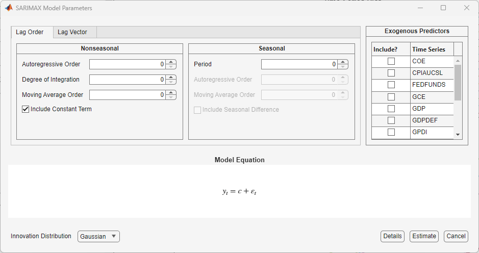
Adjustable parameters in the dialog box depend on Type.
In general, adjustable parameters include:
A model constant and linear regression coefficients corresponding to predictor variables
Time series component parameters, which include seasonal and nonseasonal lags and degrees of integration
The innovation distribution
As you adjust parameter values, the equation in the Model
Equation section changes to match your specifications. Adjustable
parameters correspond to input and name-value arguments described in the previous
sections and in the arima reference page.
For more details on specifying models using the app, see Fitting Models to Data and Specifying Univariate Lag Operator Polynomials Interactively.
What Are Conditional Mean Models?
Unconditional vs. Conditional Mean
For a univariate random variable yt, the unconditional mean is simply the expected value, In contrast, the conditional mean of yt is the expected value of yt given a conditioning set of variables, Ωt. A conditional mean model specifies a functional form for .
Static vs. Dynamic Conditional Mean Models
For a static conditional mean model, the conditioning set of variables is measured contemporaneously with the dependent variable yt. An example of a static conditional mean model is the ordinary linear regression model. Given a row vector of exogenous covariates measured at time t, and β, a column vector of coefficients, the conditional mean of yt is expressed as the linear combination
(that is, the conditioning set is ).
In time series econometrics, there is often interest in the dynamic behavior of a variable over time. A dynamic conditional mean model specifies the expected value of yt as a function of historical information. Let Ht–1 denote the history of the process available at time t. A dynamic conditional mean model specifies the evolution of the conditional mean, Examples of historical information are:
Past observations, y1, y2,...,yt–1
Vectors of past exogenous variables,
Past innovations,
Conditional Mean Models for Stationary Processes
By definition, a covariance stationary stochastic process has an unconditional mean that is constant with respect to time. That is, if yt is a stationary stochastic process, then for all times t.
The constant mean assumption of stationarity does not preclude the possibility of a dynamic conditional expectation process. The serial autocorrelation between lagged observations exhibited by many time series suggests the expected value of yt depends on historical information. By Wold’s decomposition [2], you can write the conditional mean of any stationary process yt as
| (5) |
Any model of the general linear form given by Equation 5 is a valid specification for the dynamic behavior of a stationary stochastic process. Special cases of stationary stochastic processes are the autoregressive (AR) model, moving average (MA) model, and the autoregressive moving average (ARMA) model.
References
[1] Box, George E. P., Gwilym M. Jenkins, and Gregory C. Reinsel. Time Series Analysis: Forecasting and Control. 3rd ed. Englewood Cliffs, NJ: Prentice Hall, 1994.
[2] Wold, Herman. "A Study in the Analysis of Stationary Time Series." Journal of the Institute of Actuaries 70 (March 1939): 113–115. https://doi.org/10.1017/S0020268100011574.
See Also
Apps
Objects
Functions
Related Topics
- Create Autoregressive Models
- Create Moving Average Models
- Create Autoregressive Moving Average Models
- Create Autoregressive Integrated Moving Average Models
- Create ARIMA Models That Include Exogenous Covariates
- Create Multiplicative ARIMA Models
- Modify Properties of Conditional Mean Model Objects
- Specify Conditional Mean Model Innovation Distribution
- Model Seasonal Lag Effects Using Indicator Variables
You can also select a web site from the following list:
Americas
- América Latina (Español)
- Canada (English)
- United States (English)
Europe
- Belgium (English)
- Denmark (English)
- Deutschland (Deutsch)
- España (Español)
- Finland (English)
- France (Français)
- Ireland (English)
- Italia (Italiano)
- Luxembourg (English)
- Netherlands (English)
- Norway (English)
- Österreich (Deutsch)
- Portugal (English)
- Sweden (English)
- Switzerland
- United Kingdom (English)